A comparison of Maxlike and Maxent for modelling species distributions

Merow, C., Silander, J. A. (2014), A comparison of Maxlike and Maxent for modelling species distributions. Methods in Ecology and Evolution, 5: 215–225. doi: 10.1111/2041-210X.12152

Here, the authors compare MaxLike (presence only method set up by Royle et al. 2012) to MaxEnt (widely used presence-background method). They detail how MaxEnt and MaxLike compare in their structure, providing instances of when predictions between the two would differ, and then linking the two through a discussion of sampling assumptions. The authors advocate for the use of MaxEnt’s raw output (relative occurrence rate), and point out reasons that the raw output is not equivalent to an occurrence probability (e.g., λ(x) may be larger than 1).

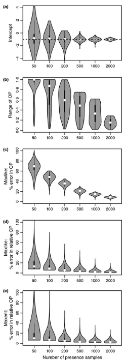
The authors further show the sensitivity of MaxLike to smaller sample sizes (Figure 3), using both empirical (Carolina wren data), and simulated data (using same model as Royle et al. 2012). MaxLike and MaxEnt outputs were strikingly similar (correlation of 0.999) when considering the raw output (relative occurrence rate) as the unit being compared between approaches. In some circumstances (low sample size), it may be difficult for Maxlike to estimate the intercept (β0) value.

In the end, the authors offer a defense of MaxEnt, and argue that both MaxLike and MaxEnt may make strong assumptions. For instance, MaxEnt assumes that the data are a random sample of individuals (though don’t both methods make this assumption?), and makes the assumption that the loglinear model is appropriate for the count data (which is defensible). Basically, if sample size is large and detection probability is constant, Maxlike is preferred since it can directly estimate occurrence probability. If sample size is small, and the model is more focused on habitat suitability instead of actual occurrence probability, the raw output (relative occurrence rate) of MaxEnt may be preferred.

 

Do Ecological Niche Models Accurately Identify Climatic Determinants of Species Ranges?

Christopher A. Searcy and H. Bradley Shaffer 2016. Do Ecological Niche Models Accurately Identify Climatic Determinants of Species Ranges? The American Naturalist 187 (4)

http://www.journals.uchicago.edu/doi/full/10.1086/685387

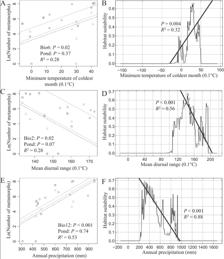
The authors examine the agreement between MaxEnt models of the California tiger salamander and known drivers of juvenile tiger salamander recruitment obtained through long term field surveys and demographic data. Climatic variable importance on juvenile recruitment was determined using an ANCOVA, where the response was the number of metamorphs, pond identity was the categorical variable, and each BioClim variable was a continuous covariate. They used model selection to determine which BioClim variables were the most important. They fit two MaxEnt models, one with randomly sampled background points and the other using a sampling bias mask to sample sites where amphibians were collected more often. MaxEnt variable importance isn’t directly comparable to their ANCOVA results, since MaxEnt will consider non-linear relationships during feature creation. They addressed this by taking the BioClim variables that were significant in the ANCOVA, and determining the linear relationship in the MaxEnt nonmarginal response curves for each BioClim covariate. If the correlation between climatic variable and either habitat suitability (MaxEnt output) or number of metamorphs (ANCOVA response variable) was of the same sign, the authors argued that it was a sign of agreement between MaxEnt models and the demographic data. They found that MaxEnt was able to find those variables most important to juvenile salamander recruitment, providing support for the use of niche models to capture aspects of species biology. They also examined some habitat suitability shifts as a function of climate projections, but I’m not going to go into that. The coolest part was their approach to quantify what they know about the population biology of the salamander species, and directly relating that to the important covariates from a niche model.

Point process models for presence‐only analysis

Renner, I.W. et al., 2015. Point process models for presence‐only analysis R. B. O’Hara, ed. Methods in Ecology and Evolution, 6(4), pp.366–379.

Renner et al. (2015) discuss the commonalities between MAXENT, PPMs, and regression for presence-only data. Using a data set on 230 presence-only locations of Eucalyptus sparsifolia in Australia, the authors highlight key ideas and benefits of PPM. A key idea in this paper was to explain PPMs as applying a regression method to point event data, and interpret the intensity (the number of presence records per unity area) as the target of interest. An important benefit of this PPM specification is that there is greater clarity around the issue of how to choose sampling points, and the possibility of querying the data being analyzed to verify that a given choice of sampling points is appropriate. In their example, they were able to show that the sampling points required for sufficient estimate convergence of the log-likelihood was closer to 100,000 that the commonly advocated 10,000 points. The reasoning for increased sampling under random sampling, as compared with survey sampling, is that it is more difficult to quantify uncertainty in the data. The authors caution that when constructing PPMs it becomes very important that you interpret what is being modeled appropriately. In particular, are you modeling intensity of sampled sites? Or intensity of individuals across a landscape? Do duplicate records exist? The authors make their data accessible from bionet.nsw.gov.au and DRYAD doi:10.5061/ dryad.985s5.

Modelling species distributions in Britain: a hierarchical integration of climate and land-cover data

Pearson, Richard G., Terence P. Dawson, and Canran Liu. “Modelling species distributions in Britain: a hierarchical integration of climate and land‐cover data.” Ecography 27.3 (2004): 285-298.

DOI: 10.1111/j.0906-7590.2004.03740.x

Pearson et. al, makes an argument that using a hierarchical framework approach for modeling species distribution benefits the understanding of unique roles and combined effects that climate change and landscape disturbance have on the determination of species distribution. The authors address the interaction between climate and land use change as determinants of species distribution by integrating both at fine scale (land cover data) with coarser scale climate data. Incorporating climate and land cover data at different spatial scales identifies the possibility that different environmental factors have a different impact on species depending on the scale. METHOD: They used presence-absence data of four plant species in Britain (which represent a range of habitat associations, life-forms, and distribution characteristics). The fine scale suitability surface was generated using the bioclimatic model SPECIES, which uses an Artificial Neural Network to first identify suitability at the European extent (continental scale – climate driven), then trained at the regional-scale (Great Britain) at 10 km then 1 km resolutions (climate and land cover driven). It is believed that at these scales these environemental factors are most apparent. Climate suitability was ultimately refined based on correlations between land cover type and observed distributions at 1 km and 10 km resolution. In order to match resolution from continent to regional scales, it was necessary to artificially aggregate suitability of cells. The hierarchical methodology was tested against a non-hierarchical method (see text) and performance of the models were evaluated using K statistic and AUC. Three threshold values were chosen (which will ultimately depend on the management situation for the species of interests).                                                                                     Incorporating land cover data improved model performance for some species, suggesting that the importance of different environmental variables on species distribution depends on the species requirements. Hierarchical vs. non-hierachichal methods (and across finer spatial scale (10 km vs 1 km)) did not perform better than the other when modeling current distribution of species. Ultimately, for predicting future species distributions, it is important to initially determine whether the decline of the species is driven from land cover of climatic variables. Theoretically, integrating hierarchical data seems like the ideal way to model species distributions, but of course there are data limitations which makes this method less feasible. It would be very interesting to apply this approach to a vertebrate/invertebrate species and compare conclusions.

On estimating probability of presence from use–availability or presence–background data.

Phillips, S. J. and Elith, J. (2013), On estimating probability of presence from use–availability or presence–background data. Ecology, 94: 1409–1419. doi:10.1890/12-1520.1

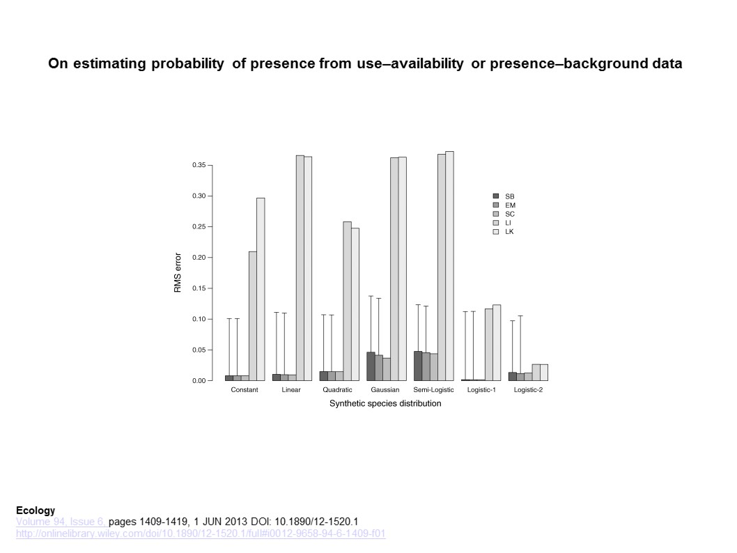
The paper investigates statistical methods (specifically logistic models) that estimates the probability that a species is present at a site conditional on environmental covariates and further addresses the disagreement in the literature on whether probability of presence is identifiable from presence-background data alone. The probability of presence is identifiable if one makes strong assumptions about the structure of the species probability of presence, however some view the assumptions unrealistic and the risk of deviating from strong assumptions can result in poorly calibrated models. An experiment (outlined below) also demonstrates that an estimate of prevalence is necessary for identifying the probability of presence. It is suggested that presence-background data must be augmented with an additional datum to reliably estimate absolute probability of presence. Methods: Seven simulated species whose probability of presence is defined by the seven functions: constant, linear, quadratic, Gaussian, Semi-Logistic, Logistic 1 and Logistic 2 (whose probabilities were bounded by 0 and 1) – which represent a variety of shapes of the response of a species to its environment – were used, in addition to randomly drawn data with 1000 presence samples and 10000 background samples chosen uniformly (0 to 1). Data was used with 5 maximum-likelihood-based methods (abbreviated as EM, SC, SB, L1 and LK) for deriving logistic models from presence-background data. Method inputs varied by 1) using a strong parametric assumption to make probability of presence identifiable (which the output failed to estimate the species probability because it fails to acknowledge species response to environment as identified in L1 and LK) and 2) requires the user to supply an estimate of the species population prevalence (as in EM, SC, SB, which was ultimately recommended to use). Based on the papers results, there is no alternative to collecting quality field work data (as opposed to making strong assumptions as in (1)) which further points out the importance to address the complexities in species-environment relationships. I thought it was pretty obvious that one cannot make strong assumptions when determining a species presence, although it might be easier for the sake of using models, but when you take an ecologist (or more specifically a wildlife manager) point-of-view determining what information goes into a model is probably more relevant.


Is my species distribution model fit for purpose? Matching data and models to applications

Guillera‐Arroita, Gurutzeta, et al. “Is my species distribution model fit for purpose? Matching data and models to applications.” Global Ecology and Biogeography 24.3 (2015): 276-292. DOI: 10.1111/geb.12268

While Species distribution models are widely used to for ecological, biological and conservation applications, researchers often lack of considerations how fit their data, model output and end-use are. SDM is flexible to be built under different types of species data, how sample process, data type, and modeling approaches influence the use of SDMs is lacking. Guillera-Arroita provided a simple framework that summarizes how interactions between data type and the sampling process may determine the quantity estimated by a SDM. They mainly talked about three types of data: presence-background, presence-absence and occupancy-detection. Our ability to deal with the probability of occupancy, the probability of site being surveyed and species detectability depend on data type being used, and this in turn determines what SDMs can estimate. By reviewing current literature and simulations, they found that even though model predictions fitted the most commonly available data, some requires estimates of occurrence probability, which is only possible with reliable absence data. When converting continuous SDM output to categorical presence/absence, it cannot clearly justify and degrade inference.


They claimed a transparent decision-making framework needs to be carried out, and people need to first formulate a clear objective. A critical consideration of using SDM is 1) whether the type of information demanded by the application in question is available, 2) whether the type of data allows unbiased estimation when used in appropriate modeling methods, and 3) thinking about the type of data that a SDM is expected to provide for a given application. This paper raises the attention for SDM users to consider whether the SDM outputs fit their research purposes, especially when continuous-binary conversion needs to be carried out. It would be interesting to see a clear decision-making framework in terms of how this kind of conservation can be justified or how to set the threshold for conversion for different ecological and conservation applications. In addition, efforts are always in demand to develop survey methods that is able to minimize the effects of the sampling process.

MaxEnt versus MaxLike: empirical comparisons with ant species distributions

Fitzpatrick, M. C., Gotelli, N. J., & Ellison, A. M. (2013). MaxEnt versus MaxLike: empirical comparisons with ant species distributions. Ecosphere, 4(5), art55–15. http://doi.org/10.1890/ES13-00066.1


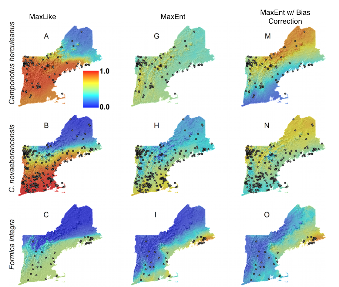
The output indices of MaxEnt are not truly direct estimators of the probability of species occurrence, but rather “ill-defined suitability [indices] (Royle et al 2012). In response to this, MaxLike, a formal likelihood model that generates ‘true’ occurrence probabilities using presence-only data, has been proposed as an alternative and shown to generate range maps that more closely match those of logistic regression models. However, it is unclear whether it can be generalized to SDMs to the extent that MaxEnt has been because the only comparison case so far used a larger sample size than is most often available, included the full geographic range of the species (and most studies cannot), and modified MaxEnt’s default settings, which may have reduced MaxEnt’s performance. As a test of generalization, Fitzpatrick et al compared MaxEnt andMaxLike models for six species of ants in New England, comparing outputs with goodness of fit, predictive accuracy measures, and comparison to expert opinion.

The authors began with 19 environmental variables, but then reduced to three: Annual Temperature and Rainfall, and Elevation. In doing so, they may have biased their study, as MaxEnt may be more robust to having multiple correlated or irrelevant variables than MaxLike. They then created 50 MaxEnt and 50 MaxLike models. The default settings were chosen for the MaxEnt models, and created a sampling bias surface based on the full dataset of ant occurrence records for 132 species was used to correct bias. Interestingly, a bias surface of all 132 species decreased MaxEnt performance, perhaps becuase the bias of the six focal species did not match that of the full dataset. Indeed, when the model was fit with a bias surface of only six species, it was a marginal improvement over the non-bias corrected models.

Goodness of fit was calculated with AIC and normalized Akaike model selection weights. Because AUC is especially problematic with presence-only data (WHY), two other measures of accuracy, minimum predicted area and mean predicted probability, were also examined. The authors have been working in this ant system for decades, so they were also able to compare models of distribution to expert knowledge and experience, a rarity, in my opinion, as many modelers are using data from systems they are unfamiliar with.

MaxLike models were better supported by the data, but model evaluation by AUC was inconclusive, although generally bias correction decreased the AUC of MaxEnt. In general, MaxEnt underestimated the probability of occurrence in areas where there were presence records, but over-estimated in unsampled areas. This is most likely due to the fact that MaxEnt assumes a mean probability of 0.5 for presence data, reducing the range of occurrence probabilities. Even with small data sets (to a minimum of five presence points) MaxLike more accurately predicted occurrence probabilities. Notably, because the authors created 50 models of each, a measure of uncertainty is available. In general, MaxLike had greater uncertainty, especially in areas with few presence points, which seems to be a fair and accurate conclusion to be drawn that machine learning methods often omit. MaxLike is able to perform better than MaxEnt on sparse data sets, even when MaxEnt is fit using default settings, and has the additional benefit of portraying uncertainty more accurately.

Comparison of occurence probabilities for MaxLike, Maxent, and Maxent corrected for sampling bias

On estimating probability of presence from use—availability or presence—background data

Phillips, S. J. , Elith, J. (2013). On estimating probability of presence from use-availability or presence-background data. Ecology, 94: 1409-1419. DOI:10.1890/12-1520.1

Ecologists studying a wide range of species wish to map species distributions and/or predict suitability of sites for occupation and persistence. This paper investigates the statistical methods that estimate the probability that the species is presence at a site as determined by environmental covariates. Exponential models are most often used for presence-background data, and provide maximum-likelihood estimates of relative probability of presence. This output is proportional to the absolute probability of presence. As the constant of proportionality is unknown models of absolute probability of presence may be preferable. Five logistic methods (LK, LI, SC, EM, SB) for using presence-background data are presented and tested in an experimental comparison. Seven simulated species with defined probability of presence functions were modeled in an environment with a single predictor variable ranging from 0-1 uniformly across the landscape. For models that required an estimate of prevalence, the known simulated presence was used first followed by the true prevalence with an error of 0.1 to assess the sensitivity of the estimate. There was a stark contrast between two groups of models with LI and LK methods (no species prevalence parameter) having higher RMS errors than the SC, EM, SB methods (includes species prevalence parameter). The EM, SC, SB methods performed well in the experiments given an estimate of prevalence. These models may be useful as they can estimate the absolute probability of occurrence at a location, which can aid in the management and conservation of species across a region. Due to the potential of over- or under-prediction with a substantially incorrect estimate of prevalence, in cases were estimates of prevalence are unreliable the use of MaxEnt, or other methods like it, may be better.i0012-9658-94-6-1409-f01_10.1890_12-1520.1

The landscape configuration of zoonotic transmission of Ebola virus disease in West and Central Africa: interaction between population density and vegetation cover

Walsh, M. G., & Haseeb, M. A. (2015). The landscape configuration of zoonotic transmission of Ebola virus disease in West and Central Africa: interaction between population density and vegetation cover. PeerJ, 3(1), e735–13. http://doi.org/10.7717/peerj.735


Following the epidemic outbreaks of Ebola Virus Disease (EVD) in West Africa in 2014, it is obvious that the ability to predict, and perhaps even prevent, such outbreaks could greatly inform public health efforts, and save lives. Walsh & Haseeb (2015) use a point process distribution model to understand what are the socio-ecological drivers of zoonotic transmission events of EVD. Unique transmission events were recorded from the PubMed Database and World Health Organization reports, and matched to a geographical location. The authors chose three types of covariate data: WorldClim data on temperature and precipitation, Maximum Green Vegetation Fraction from Modis as a measure of vegetation, or forest, cover, and population density data from the Global Urban-Rural Mapping Project. First, they created a homogenous Poisson process (ppm), which served as a null model because the expected number of location points scaled with the area of the subregion, and inhomogenous Poisson process, which incorporate spatial dependence into the location of transmission events. The inhomogenous ppm fit the data better, and then was then expanded to include the four covariates listed above, plus altitude and an interaction covariate between vegetation cover and population density. The ppm allowed for the use of conventional statistical tests of significance, such as p-values and confidence intervals. Three covariates came out as important. Both increasing population density and increasing vegetation, although slightly less so, cover corresponded to a decrease in spillover risk. Interestingly, the interaction between these two variables was also significant, implying that the ‘protective effect’ of vegetation cover decreases with increasing population density. This suggests the presence of ecotones, where denser human populations are coming into contact with recently fragmented forest, an avenue for zoonotic spillover that has been suggested in the past.

Thoughts: An ecological niche model of EVD has been described previously, but this study incorporates the additional complexity of social factors, which I believe is especially important when considering spillover events. Doing so, however, removes distribution modeling from this idea of a fundamental niche, in my opinion, because it is no longer simply where EVD can persist but where it spills over. Semantically, this could be a ‘niche’ for spillover events. I also think it is important that they considered interactions amongst environmental covariates, especially because certain variables are correlated or depend on others.

The study’s code is online with data, if anyone is interested in reproducing it or just playing around point process models.

Mapping species distributions with MAXENT using a geographically biased sample of presence data: a performance assessment of methods for correcting sampling bias

Fourcade, Y., et al. (2014). “Mapping species distributions with MAXENT using a geographically biased sample of presence data: a performance assessment of methods for correcting sampling bias.” PLoS One 9(5): e97122.


http://journals.plos.org/plosone/article?id=10.1371/journal.pone.0097122


Fourcade et al. attempt to assess the effectiveness of a number of methods for correcting sampling bias in species distribution modeling with MaxEnt. Bias in species sampling has been well established as an important and difficult problem in species distribution modeling. The authors take large, and likely spatially unbiased, presence only sample sets for 1 virtual and 2 real species and impose 4 types of spatial bias on them to simulate sampling bias. These types of biases are (1) Two Areas, the northern region has high sample density and the southern region low density, (2) Gradient, a density gradient decreasing from north to south, (3) Center, the density decreases gradually from the core of the distribution to the edges, (4) Travel Time, probability of keeping a record was highest when it had the lowest travel time to the nearest city. 5 different data-processing methods were used to limit the effect of these spatial biases: (a) Systematic Sampling, a grid of a defined cell size was superimposed on the distribution and 1 record was chosen per grid cell, (b) Bias File, MaxEnt can be given a file representing sampling effort with which it weights the sampled points, (c) Restricted Background, MaxEnt’s background points were drawn exclusively from buffer areas around biased occurrences, (d) Cluster, a PCA was performed on the environmental predictors then occurrence points were analyzed for clustering in the 2 dimensional environmental PCA space and 1 record was randomly sampled per cluster, (e) Split, occurrences were split into a northern and southern group and MaxEnt was applied independently to each area. These methods all seem relatively well grounded individually but the combination fails to make much sense. Most notably, it is entirely unclear why grid based selection is used for spatial thinning and cluster analysis for environmental thinning. Models were compared using AUC, overlap species probabilities in environmental (Denv) and geographic (Dgeo) space. Biased models invariably had lower AUCs than unbiased models and clearly deviated from the unbiased model by all measures. Decrease in AUC, however, was small and the AUC of biased models was usually still in the range generally accepted as a well fit model. The effect size of each bias type depended on the species and evaluation method. The authors focused on Dgeo (Denv was strongly correlated) as the main measure of effectiveness of bias correction. Overall only 29% of all combinations (species*bias type*bias intensity*correction method) showed improvement over the biased model with the simulated species substantially easier to correct (57% were successful corrections). Restricted Background (c) failed in almost all cases (6% successful). All other methods performed better but were differentially ranked depending on the combination of factors. Systematic sampling (a), though not always ranked first, performed most consistently and slightly better overall than the competing methods (33% successful). Bias file (b) and cluster (d) methods sometimes outperformed Systematic Sampling but were slightly less successful overall (23%, 23%). Probably the most important result of this work is the bad performance of the Restricted Background (c) method, as it seems to be consistently used/recommended when fitting MaxEnt to biased data. Though Systemtatic Sampling (a) performs well and consistently, the authors acknowledge that the second main conclusion is that the best way of handling bias is often context specific and so one ought to attempt multiple different correction methods in practice. Their somewhat strangely chosen set of correction methods further reinforces this point as other methods that have been demonstrated as effective went untested or were replaced with minor variants that may have changed their effect.


Fourcade et al.,