Estimating patterns of reptile biodiversity in remote regions

Ficetola, Gentile Francesco, et al. “Estimating patterns of reptile biodiversity in remote regions.” Journal of Biogeography 40.6 (2013): 1202-1211.


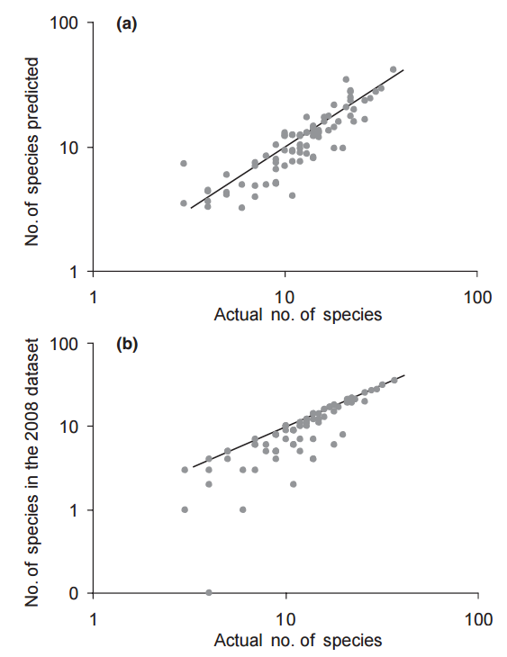
The authors aim to predict species richness of reptiles (turtles, amphisbaenians, and lizards) in the Western Palaearctic using Bayesian autoregressive models (BCA) and spatial eigenvector mapping. They used these methods to account for the significant amount of spatial autocorrelation in their predictor variables. They considered accesssibility (travel time to nearest city with population > 50000 people), density of protected areas, and environmental covariates as their predictors of species richness, where richness was count data with an assumed Poisson error distribution. They argued that accessibility was a layer that got at sampling and collection biases. Further, they argued that spatial resolution could influence predictions, so they predict at 1 degree squared and 2 degree squared resolution. Further, they transformed nearly all of the predictor variables, which I can’t really tell if they needed to based on the modeling approach. Models were validated by comparing predicted species richness to data from exhaustive sampling on a subset of the spatial cells. Accuracy was computed by comparing outputs of 3 linear models of predicted versus actual richness values (1. actual ~ predicted, 2. actual ~ recorded richness until 2008, 3. actual ~ intercept). BCA models were qualitative similar to the spatial eigenvector approach, and the BCA models predicted species richness with high accuracy.

Moving beyond static species distribution models in support of conservation biogeography

Franklin, Janet. “Moving beyond static species distribution models in support of conservation biogeography.” Diversity and Distributions 16.3 (2010): 321-330.

DOI: 10.1111/j.1472-4642.2010.00641.x

SDM extrapolates species locations in space based on correlations of presences with environmental variables. Nonetheless, most of the SDM are static, assuming species locations data used for modeling are representative of its true distribution, and distributions are in equilibrium with environment factors. In order to meet the needs of conservation biogeography, static SDM needs to move to incorporate dynamic processes determining species distribution. Franklin therefore discussed three strategies of increasing complexities for SDM incorporating process models, namely 1) to incorporate models of species migration to understand the ability of species to occupy suitable habitat in new locations; 2) to link landscape disturbance and succession to suitability; 3) to link suitability models with habitat dynamics and population dynamics. Generally, migration models account for species dispersal and establishment, but not account for interactions with other species. Both population viability models and community dynamics models account for dispersal and competition. However, there will always be trade-offs between using complex, mechanistic versus simple, empirical models for environmental change forecasting. By linking all modeling complexities, the framework could be powerful to understand the potential interactions and population persistence. But good knowledge of species interactions and life history is required. Most notions in this paper are at conceptual level, though he brought up a really good point to combine dynamics into SDM. However, in many cases we use SDM is to compensate for our lack of knowledge on the ground. Hopefully we can see some specific applications that include dynamic variables into species commonly used SDMs, and maybe a comparison can be made in terms of which model is more compactible with dynamic processes.

Overcoming limitations of modelling rare species by using ensembles of small models

Rare species distribution modeling is inherently difficult due to the issue of relatively low number of occurrence points relative to a high number of explanatory variables. To alleviate this difficulty a researcher could reduce the number of predictor variables used in the model such that the ratio of predictors to occurrence points is 1:10. This method can be problematic for extremely rare species where 20 occurrence points would only allow for two predictors. Additionally, there is an elevated interest in modeling distributions for rare species due to the conservation interests of these species. The mismatch between the need to model rare species distribution and the difficulty in doing so is termed the “rare-species modeling paradox.” A method in which many models containing a few predictors are created and then averaged according to weighted scores based on model performance has been proposed to get around the difficulties of modeling the distributions of rare species. This method, called an ensemble of small model (ESM), was applied reasonably well to a single endemic species of the Iberian Peninsula, but had yet remained untested against traditional species distribution models (SDM). This paper looks at how ESMs compare traditional SDMs for 107 species of varying rarity. 107 species of vascular plant were selected for this analysis and split into three groups, very rare, rare, and less rare. GLMs, GBMs, Maxent, and their ensemble prediction (EP) were constructed for all species using 11 predictors. A linear mixed effects model was used to test for the effects of modeling strategies (ESMs, traditional SDMs), modeling techniques (GLM, GBM, Maxent, EP), sample size, and the two way interaction between the factors. The linear mixed effects model showed that ESMs nearly always outperformed their standard counterpart. The effects of all factors on model performance was significant. Modeling strategy interacted with sample size, where species with a low sample size (very rare) benefitted the most from the use of ESMs. This paper shows that ensembles of small models can be an effective way for modeling rare species. This study was conducted using only vascular plants and the method will need to be tested on other taxonomic groups to prove validity, though the authors anticipate similar success when implemented.

Breiner, F. T., Guisan, A., Bergamini, A., & Nobis, M. P. (2015). Overcoming limitations of modelling rare species by using ensembles of small models. Methods in Ecology and Evolution, 6(10), 1210-1218. DOI: 10.1111/2041-210X.12403


Effects of incorporating spatial autocorrelation into the analysis of species distribution data.

Dormann, Carsten F. “Effects of incorporating spatial autocorrelation into the analysis of species distribution data.” Global ecology and biogeography 16.2 (2007): 129-138.

This review paper investigates the importance of incorporating the effects of of spatial autocorrelation (SAC) into any species distribution model. The author was interested in answering two questions. First, does SAC the parameters estimated from species distribution data? Second, does incorporating SAC increase model performance?

The literature review was conducted using Web of Science, search methods the author believed to be reasonable to handle SAC included the following: autologistic regression, generalized least square regression, and correction of significance levels. The search parameters provided to web of science were: “spatial autocorrelation” and “ecology or distribution”, additionally the author would review any papers not returned through Web of Science, but cited in a paper found through the search criterai. The inclusion criteria were: (1) a species distribution was analyzed (2) presence of a traditional analysis (GLM or GAM) and spatial model (3).

Information extracted from the reviewed studies.

Arrangement of samples

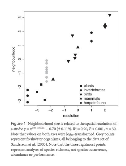
Size of neighborhood

Spatial extent/grain

Type of autoregressive function

Species/group

Quality of SAC removal/control

Response variable

Model coefficients

Statistical methods

Importance of SAC

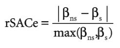
To measure the effect of correction for SAC the following equation was provided. Where S stands for spatial coefficients and NS stands for non-spatial coefficients.

rSACeDoorman2007

The effect of correcting for SAC on overall model quality was quantified with AIC, R2, and deviance-based pseudo-R2.

Findings from this study indicate that there was no difference in response type for single species studies in terms of rSACe. The author did find an effect for the range of spatial autocorrelation (neighborhood) and spatial resolution. Meaning that when controlling for the effect of spatial resolution in the study, the effect of SAC was significant. For the effects of spatial autocorrelation on model quality, the author observed a significant improvement in AIC values when SAC information was provided to the model.


Dorman2007

Support vector machines for predicting distribution of Sudden Oak Death in California

Guo, Qinghua, Maggi Kelly, and Catherine H. Graham. “Support vector machines for predicting distribution of Sudden Oak Death in California.”Ecological Modelling 182.1 (2005): 75-90.

Recently, several types of oak trees in California have been severely impacted by the emergence of Sudden Oak Death, an infectious disease caused by the pathogen Phytophthora ramorum. Using  support vector machine (SVM) approach, researchers provide a prediction for the distribution of sudden oak death with both two class and one class svms.

Researchers argue that a presence only modeling approach, with SVM as an example, will increase the prediction accuracy compared to methods that use a pseudo-absence approach  drawn from the underlying distribution of the presence data. Traditionally, SVMs were designed for two class classification for positive and negative or presence and absence for SDM purposes. However, true absence data is often hard to come by. However, a one class, presence only approach, will have a harder time detecting which environmental features are important in predicting the outcome. To overcome this a one class SVM approach was developed.

The training data for this paper consisted of locations where the occurrence of P. ramorum was confirmed in oaks located in California. Host distribution was generated through Landsat ThemP analysis project which provides information at a fine spatial scale (1:100,0000). 14 Environmental variables were used to train the models, environmental information was provided from Daymet. A five-fold cross-validation method was used to evaluate model accuracy.

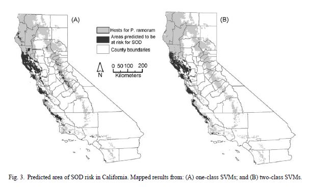
SuddenOakDeathFigure


Researchers reported the true-positive rate for your one class SVM was 0.9272 + 0.0460 over an area of 18,441 km2. For the two class SVM reported a true-positive rate of 0.9105 + 0.0712 with a predicted area of 13,828 + 1316 km2. One class SVMs have two main advantages compared to other presence only modeling approached. First, they are able to utilize unique shapes of distributions in feature space through kernel functions. Second, one class SVMs make no assumptions about the distribution of the environmental parameters. Differences in the predicted areas between the two models may indicate that either the one class model has over predicted the area or risk or the two class model has underpredicted. Observed differences can be explained by the higher-true positive rate from the one class model, often false positive rates will increase with the true-positive rate. Another reason for larger risk areas in one class models can be attributed to the two-class model sampling pseudo-absences from presence points, resulting in a more conservative risk estimation. This study demonstrates how a support vector machine approach can be used to ascertain the potential risk of an infectious disease epidemic.

Do Ecological Niche Models Accurately Identify Climatic Determinants of Species Ranges?

Searcy, C. A., & Shaffer, H. B. (2016). Do Ecological Niche Models Accurately Identify Climatic Determinants of Species Ranges? The American Naturalist, 187(4), 1–13. http://doi.org/10.5061/dryad.667g2


A major question surrounding ecological niche modeling is if models accurately reflect the biological ranges of species and if they are informative regarding a species niche requirements. If they do reflect these ecological “truths”, and not simply correlations with climatic variables, then their use in the prediction of species ranges into future climatic conditions is valid. To explore this issue, Searcy & Shaffer (2016) compare climatic variables that determine recruitment in the field with those predicted as high ranking by MaxEnt. Using two decades of demographic data on the endangered California Tiger Salamander, the authors replicated BioClim variables using climate data from nearby weather stations and ran ANCOVA models to measure how well a climatic variable correlated with juvenile recruitment of the salamander. They then created two MaxEnt models:
– a basic model that used permutation importance to rank variable importance
– an informed model that used permutation importance and percent contribution to rank variable importance, and
– corrected for sampling bias
– limited background points based on natural history of the species
– used model selection to select the model’s regularization multiplier

They then compared the variable importance rankings from the ANCOVA models to the two MaxEnt models, evaluating ranking and the response curves, the latter to see if the relationship between the variable and habitat suitability/recruitment was the same.

They found six variables to be highly correlated with recruitment, and these six variables were highly correlated with those predicted as important by MaxEnt, when using the informed model with importance by permutation. Notably, this was not seem with the other models, suggesting that an informed model using permutation may best illustrate biological realism. Interestingly, the response curves were not all the same, with temperature variables exhibiting similar response curves, but precipitation variables correlated in opposite directions. This may be due to the fact that they only considered linear responses, effectively dropping most MaxEnt curves, which were non-linear. It may also be due to the temporal scale of rainfall, in which one year with above-average rainfall can lead to high population growth, but an overall increase in rainfall over many years can decrease population growth.

In general, this paper provides evidence that ENM is based on biological realism, albeit with several caveats. Only the informed MaxEnt model with permutation reflecting this conclusion, suggesting that variable ranking by permutation should always be chosen, and models should be corrected for sampling bias and natural history, and controlled with a regularization multiplier. It also stresses that many biological responses are non-linear, so any models that treat them as such are likely to fail.

Note: They also use the MaxEnt model to predict the effect of climate change on the salamander, but this seemed less relevant and generalizable to the class, so I didn’t report on that aspect.

Eight (and a half) deadly sins of spatial analysis

Hawkins, B.A., 2012. Eight (and a half) deadly sins of spatial analysis. Journal of Biogeography, 39(1), pp.1–9.

Hawkins argues that many ecologists are of the understanding that the existence of spatial autocorrelation is a bias or artifact of sampling that must be removed rather than embraced when trying to model their distribution. In this opinion essay, he argues against this notion as well as against eight (and a half) other commonly held perceptions in ecology. First, spatial autocorrelation is not bias. Instead this autocorrelation in nature is what we wish to understand. Indeed, spatial autocorrelation in nature is separate from residuals in a model. Second, spatial regression is not always the best according to Hawkins and some statisticians. In the Beale (2010) paper that we read, we did see that OLS produced estimates that were not all that different from spatial models and here, Hawkins notes that even when studies find that spatially explicit model are best arise in simulation studies of species rather than using real data. Thus, muddying the waters for making generalized claims about how spatial models are always better. Third is the assumption of stationarity among the entire landscape. Authors often fail to report whether or not they have determined whether their data abides by this assumption. Fourth, Hawkins argues that partial regression coefficients are not very meaningful for these contexts. The main idea of this section is just that we can’t quibble over which particular type of multiple regression, and values of coefficients, is the best method for understanding a process. Fifth, was correlation does not equal causation and argues that although many ecologists have heard this mantra, some still don’t uphold the value of the statements. Sixth was the idea that species richness causes bias. Hawkins emphasizes that if the species is prevalent in an area, we should not wish to remove this phenomenon from our data. Usually, he states, this type of misconception is due to a confusion of precision with bias. Next, he argues that spatial processes explain spatial patterns (i.e. there are biological processes operating in a spatially structured environment that we wish to understand). Finally, he notes that spatial autocorrelation causes red shifts in regression models. This means that there is an over-estimation of importance of broad scale predictors in OLS multiple regression models. He argues that this point is not important at all. Take away points from this paper include: (1) that we should not try too much to focus on methodology when describing species distributions. If we do this then we run the risk of trying to capture all complexity in our data rather than understanding it. (2) Many of the disagreements among researchers using multiple regression tools stem from the lack of understanding of the assumptions that these models make. Although I agree with his findings about understanding assumptions and autocorrelation for multiple regression models, I find it difficult to validate his opinions on all matters of these subjects because he lacks citations backing up his claims.

Modelling ecological niches from low numbers of occurrences: assessment of the conservation status of poorly known viverrids (Mammalia, Carnivora) across two continents

Papeş, M. and Gaubert, P. (2007), Modelling ecological niches from low numbers of occurrences: assessment of the conservation status of poorly known viverrids (Mammalia, Carnivora) across two continents. Diversity and Distributions, 13: 890–902. doi:10.1111/j.1472-4642.2007.00392.x


In order for a species to occupy their ecological niche that abiotic and biotic conditions need to be favorable in addition to being geographically accessible. These niches are most often modeled with the most common data – present records, but this data has plenty of issues including unknown sampling holes, linking time of collection with abiotic factors, biased geographical sampling, and geo-referencing museum specimens. Poorly studied species have the additional challenge of low sample size, which exacerbates the previous issues and may also biased sampling of environmental space. Previous studies have shown ENM with small sample sizes performance are dependent on model and variable choice, machine learning does better. The authors use this discrepancy and model performance to motivate the comparison of GARP to the (at the time) newer modeling approach of MaxEnt.

Models were compared for 12 species. The current state of was collected from museums specimens, which were geo-referenced. All 19 Bioclim variables were used at the 4.5 km resolution. The default values were used for MaxEnt and along with linear features. In the case of N>10 quadratic features were also used. GARP, a machine learning methods, used 50% of the data to produce 200 to 500 models. The remaining 50% of the data was used to test model performance; the 10 models with the lowest false-negative rate were kept. Outputs of each modeling approach were compared using zonal statistics. The ecological niche models were combined with land-use and current reservation/conservation status.

MaxEnt and GARP models had general positive association – but not a strong trend (Figure 1). In other words, they had similar distributions but very different means. MaxEnt predictions’ were broader than GARP, the reverse of expected (Figure 2 and 3).

Consequences of spatial autocorrelation for niche-based models

SEGURADO, P., ARAÚJO, M. B. and KUNIN, W. E. (2006), Consequences of spatial autocorrelation for niche-based models. Journal of Applied Ecology, 43: 433–444. doi: 10.1111/j.1365-2664.2006.01162.x

Spatial autocorrelation is an important bias source in most spatial analysis. Segurado, Araujo and Kunin (2006) examined the bias caused by spatial autocorrelation based on explanatory and predictive power of niche-based species distribution modes. Two kinds of freshwater turtle and two simulated species were used to construct SDM using generalized linear models (GLM), generalized additive models (GAM) and classification tree analysis (CTA). In general, GAM and CTA outperformed GLM, though all of them are vulnerable to the effects of spatial autocorrelation, which leads to an inflation effect up to 90-fold. Efforts for reducing autocorrelation effects included systematical subsampling and inclusion of a contagion term. Subsampling was only partially successful in avoiding inflation effect, whereas the inclusion method fully eliminated or sometime even overcorrected the effect. Based on this study, they recommended to implement techniques and procedures like the null model approach in order to improve niche-based SDM performance. However, their discussion is limited only to univariate modeling. When more then one candidate variable to predict SDM, a more complex assessment needs to be considered. However, since SDM are usually multivariate, their conclusion may still be able to offer informative rules, but to which level autocorrelation will affect SDM, or which model perform better may need further exploration.

Inference from presence-only data; the ongoing controversy

Hastie, T. & Fithian, W., 2013. Inference from presence-only data; the ongoing controversy. Ecography, 36(8), pp.864–867.

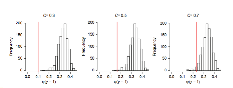
In response to Royle et al. (2012), Hastie & Fithian (2013) question whether it is possible to estimate the overall species occurrence probability, or prevalence, given presence only data. The main concern with Royle et al. (2012) is their assumption of parametric form for nearly log-linear variables. Problematically for most real world data, the functional forms are almost never linear. Royle et al. (2012) approach of linear approximation is a useful simplification that allows researchers to estimate prevalence. But Hastie & Fithian (2013) argue that these assumptions are too arbitrary to be robust in practical settings. However, by assuming this, MLE methods can be used to estimate species probability of presence. To illustrate this point, they simulate nearly linearly logistic data and fit a linear logistic model using likelihood values to generate a large sample of values of x (geographic sites representing a unit of area), via the uniform distribution of sampling to determine presence/absence points. Next, they subset 1000 values of x’s, which had the species present. Figure 2, shows results from three separate simulation runs with the red line showing the true value for the species occurrence probability. In all cases, the values of the histogram bear no relationship to the true values of probability of presence. This paper clears up the main argument against using presence-only data to calculate the full support of species prevalence.