Tag: Ashton Griffin

Sandve, Geir Kjetil, et al. “Ten simple rules for reproducible computational research.” PLoS Comput Biol 9.10 (2013): e1003285.

Link

Scientific research has seen a rise in recent years of the increasing demands for more computational skills required to conduct biological and ecological research. This increase in research complexity has precipitated the need to stress the importance of reproducibility of computational methods. Reproducibility is an abstract concept that provides a way to consider how likely someone else provided your data and methods could recreate the results reported in your manuscript. Provided in this paper are ten simple rules that every researcher should consider when conducting a computational based experiment.

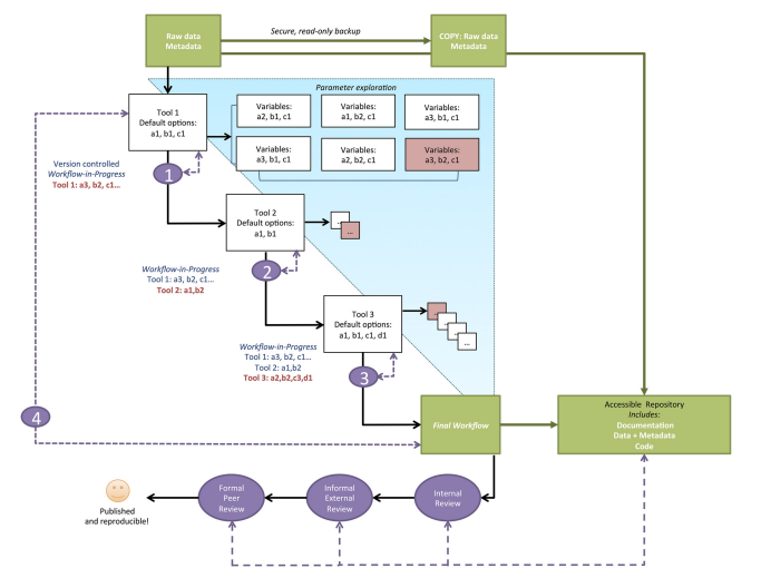
First, provide information regarding how every provided result was produced, even if the result ends up not making the final draft. This will not only help recreate the results reported, but also provide insight into the parameter selection process. Secondly, avoid manual data manipulation steps when possible. Data manipulation is a feature of almost any study; however, manually editing data is something that can not be easily recreated with a script. Third, make backups of software versions used in analysis. Packages and programs are updated constantly, and sometimes updated one package may break its dependencies on another. Currently, researchers can use docker as a means to save current software versions. Fourth, version control all custom scripts. This is related to the fourth rule, by version controlling your scripts you are increasing the likelihood that the script will be able to run in the near future. Fifth, keep track of intermediate results. This will help should you ever need to return to an intermediate step in your analysis and make corrections. Sixth, make notations for how to recreate stochastic data. If you induce random noise into the data it’s best to provide the parameter values governing how the noise is manifested.  Seventh, store the data behind plots. This cuts out the need to rerun potentially time consuming analysis. Eighth,  in your final script save data outputs at identifiable milestone markers within your analysis. Ninth, Where possible provide information regarding why you selected for certain parameters or methods instead of others. Lastly, upload your scripts and data into public domain for ease of access to other researchers.

Shade, Ashley, and Tracy K. Teal. “Computing Workflows for Biologists: A Roadmap.” PLoS Biol 13.11 (2015): e1002303.

Link

 

This paper provides a computational framework for biologist in an effort to speed up the development of computational skills needed in contemporary biological research. Broadly the roadmap provided can be broken down into two categories based on within group review and external review. The first step in the computational workflow is to create backup copies of the raw data and metadata and make notes on any data filtration applied before receiving the data. Next, the researcher will want to identify her goals of the study and distinguish whether or not she is conducting a hypothesis test or data exploration. After the goals are properly identified the researcher will want to consider the parameter space which is comprised of all decisions involved in modeling the data (including program selection). Authors encourage adapting branching pattern approach at this point and evaluating parameter space in three key areas: sensitivity analysis, sanity check, and control analysis. Sensitivity analysis observes how model outputs change with change in input options. Sanity checks are inquiring if the model outputs are what the researchers expect to observe or do these results make biological sense. Control analysis uses simulated or provided data to have a firm understanding of the employed model. At certain points in the workflow the researcher will want to conduct reproducibility checkpoints by making sure that given a clean start they can recreate the current step in their analysis. Lastly, researchers will want to utilize online repositories to both backup their data and solicit outside feedback in their approach.

 

Williams, Gareth J., et al. “Predictive modeling of coral disease distribution within a reef system.” PLoS One 5.2 (2010): e9264.
Link

This study uses a boosted regression tree approach to determine relevant factors involved in predicting the spread and Porites growth anomaly and Montipora white syndrome. Boosted regression trees are similar to additive regression models in that the terms considered are decision trees that are fitted with a forward selection process. BRTs provide two key insights from their analysis. First, they demonstrate the underlying relationship between response and predictors and second that establish which predictor has the most influence on the response.

Over two five-week periods (October 2007 – November 2007 & May – July 2008), a disease surveillance survey was conducted within the Coconut Island Marine Reserve. Coral species that were considered important to the local reef community were assessed in their current health status with respect to presence or absence of known coral diseases. Belt transect surveys were used in order to quantify the amount of disease prevalence, and classify the status of observed disease lesions. Environmental factors were collected by either deployed data loggers and observation of biological factors (eg: fish predation) by experts participating in transect surveys. Given the low sample size within the data set, researchers opted for a 10-fold cross-validation for assessing model performance.

 

Results indicated that Porites Growth Anomalies (PorGA) were primarily negatively correlated with turbidity and depth. Porites tissue loss (PorTL) was driven by fish abundance, temperature and turbidity. Porites trematodiasis (PorTrem) was associated with colony density, fish abundance, depth, and colony cover. Montipora white syndrome (MWS) was associated with juvenile parrotfish abundance and positive correlation chlorophyll-a. Its interesting how little influence temperature had on disease prediction given how temperature is an established driver for other coral syndromes (eg: bleaching).

 

Naimi, Babak, et al. “Spatial autocorrelation in predictors reduces the impact of positional uncertainty in occurrence data on species distribution modelling.” Journal of Biogeography 38.8 (2011): 1497-1509.

Link

This study investigates how using information regarding spatial autocorrelation of environmental variables can help mitigate the error introduced from positional uncertainty in species occurrence data. Spatial autocorrelation refers to the idea that for any given point in space of an environmental variable one would expect the nearby surrounding points to be more similar compared to those that are further away. Position uncertainty results from errors in determining where the geographical occurrence of the observation took place. In this study researchers used a simulated data set to observe how the interactions between spatially autocorrelated variables and positional error can influence the predictions made in both presence-only and presence-absence SDMs.

The simulated artificial data set was comprised of 2 environmental variables and one set of species observations that was linked to the environmental gradient. Researchers incorporated errors into their observation data based on a normal distribution, and then further propagated the uncertainty with Monte Carlo simulations. Species distribution models were evaluated using AUC and Cohen’s Kappa statistics. Cohen’s Kappa is a proportional measure that is variable to the set threshold detection level (unlike AUC). A two-way Friedman’s test was employed to asses if SAC in predictors reduced the influence of positional uncertainty.
Results showed that model performance varied depending on the trade between the degree of positional uncertainty and spatial autocorrelation in the provided data set. It is possible for spatial autocorrelation to reduce the impact of positional error; however, it is unable to fully compensate for error when positional error is extreme. Boosted regression trees, Generalized additive models, and Generalized linear models all outperformed random forests, Garp, and Maxent in terms of AUC. This is explained by the fact that the better performing models are presence-absence and thus have more information to make their predictions on.

Link

This study compared the likelihood functions used in species distribution modeling that have differences in occurrence records such as presence-only, presence-background, and presence-absence. Specifically, researchers focus on the differences of point and count data. Results indicate that the differences between the likelihood function of count data, and the likelihood function for point methods can originate from the same underlying inhomogeneous Poisson point processes model.

To first accomplish this, researchers provide an equation that allows for the consideration of continuous environmental space instead of discrete environmental space (equation 1). Researchers then adapt geographic space from discrete to continuous. They then provide considerations for the response type given either a discrete or continuous environmental/geographic space. After addressing these points, researchers then present the likelihood functions for unconditional inhomogenous Poissoin point processes and conditional inhomogenous Poisson point processes, and indicate how both functions are related to the Poisson log-likelihood.  

To asses how parameter estimates might vary across different realizations of the species range, researchers conducted a simulation and compared differences between IPP and logistic regression using either 100 or 10,000 availability points and one spatially autocorrelated environmental variable. To generate different parameter estimates the creation of environment and occurrence observation was repeated roughly 500 times. The mean estimates were compared to the true values; as well as, using Monte Carlo standard deviations. Most models were able to capture the true parameter value; however, the Poisson GLM performed poorly compared to all other models. The reason provided is because the scale the environmental covariate was distributed was much smaller than the resolution of the grid cells.

 

Dambach, Johannes, and Dennis Rödder. “Applications and future challenges in marine species distribution modeling.” Aquatic Conservation: Marine and Freshwater Ecosystems 21.1 (2011): 92-100.

Link

This study highlights how the effects of climate change are altering marine species distributions and also highlights challenges unique to marine species distribution modeling. Researchers posit that increasing ocean temperatures will force species to shift either in latitude or depth with accompanied tradeoffs with respect to the selected shift. As a consequence invasions and local/global extinctions are expected to continue to increase.

Authors provide three points highlighting unique challenges within marine species distribution modeling. First, authors consider how complex three dimensional structure generates the need to understand how depth influences contributing factors. Related to the three dimensional complexity issues is that preference in depth can differ depending on the life stage of the species in question (eg: larval and adult stages). One possible solution is to apply species distribution models at varying stages of depth, then layer predictions appropriately. Second, dispersal via ocean currents is a significant driver of many marine in some instances more important than local physical properties themselves. Lastly, there exists a known bias in occurrence records between coastal and open water surveys. Which can complicate knowledge of habitat preference for species that occupy both at some point in their life cycles.

This paper also presents a case study on great white sharks, Carcharodon carcharias, habitat suitability. The great white shark is a suitable organism to model due to its known global migration patterns. White shark occurrence records were accessed through GBIF. Environmental parameters considered were the following: minimum depth, sea-surface temperature, and salinity. Researchers used MaxEnt and a Last Glacial Maximum output to determine how white shark distribution could change under climate change. Outputs suggest that white sharks are more likely to adjust their distributions to increased latitudes in the future due to changes in environmental conditions. Given that the white shark is an apex predator this could further create consequences for other animals currently occupying the predicted expansion areas.

Ficetola, Gentile Francesco, et al. “How many predictors in species distribution models at the landscape scale? Land use versus LiDAR-derived canopy height.” International Journal of Geographical Information Science28.8 (2014): 1723-1739.
Link

In this study researchers employ an approach to better evaluate which features of the landscape, mainly those measured by remotely sensed tools, are important for a selected bird sanctuary in the Netherlands. They define their study as being small with no variability in climatic or topographic gradients, which provides reason to suggest that features of the landscape are driving species distribution. Using data collected from a Biodiviersity Multi-SOurce Monitoring System: From Space to Speices (BIO_SOS) project, researchers compared the performance of five different models in explaining species distribution provided a fine scale study area.

 

Models

1. Models using a relatively large number of traditional land-use variables
2. Models using a small number of land-use variables
3. Models excluding land-use variables, and only using canopy height collected via LiDAR sensors
4. Models using a large number of land-use variables and LiDAR
5. Models using a small number of land-use variables and LiDAR

 

Occurrence data was collected within the Veluwe located in the Netherlands, the Veluwe is roughly equivalent to a national park found within the United States. Land-use/land-cover data sets were collected through the Dutch government, and the likely satellite system used to collect the base images were Landsat. Seven classified habitats were included in this study: broadleaved forest, coniferous forest, heathland, grassland, sparse vegetation, built-up, and shifting sand. The study area was partitioned into 20 m x 20 m cells, and for each cell researchers measured the average cover of habitat within a 100 m radius from the cell center. LiDAR data was also attributed to cells in the same way.

For Analysis, researchers first determined the correlation coefficients between independent variables with |r| >0.7 as a cut off. They also used a variance inflator factor to determine whether multicollinearity occurs in developed models. MaxENT models were built for predicting species distribution.

Results indicated that in general there was a lack of collinearity between environmental variables (|r| < 0.7), with the exception of canopy height being positively related to coniferous forests and negative to heathland and a negative relationship between forest and heathland. Seven out of the nine species of birds evaluated using MaxENT were found to be best predicted using LiDAR provided information with the majority of models performing best with LiDAR only information. This finding suggest that increased detail in provided environmental information (eg: LiDAR) will provide, in general, better fit models for predicting species distributions. Provided the measured environmental information is relevant to predicting the occurrence of the focal species.

Article

Findings from Olden 2002, Predictive models of fish species distributions: a note on proper validation and chance predictions, points to that fact that there is a critical need for a method to evaluate whether or not SDM predictions would differ from what would be expected from chance alone. This paper provides a null-model in an attempt to address the ideas outlined in Olden 2002. Researchers point out that a major drawback to AUC in pseudo-absence approaches is that the AUC value indicating a perfect fit is not 1 but instead 1-a/2. Where a is the fraction of the geographical area of interested covered by a species’ true distribution which is typically an unknown quantity.

Developing the null model for evaluating AUC estimates.

1. Determine the AUC value of the real SDM from provided data.
2. Generate a null model by randomly collecting localities without replacement from the target species supposed distribution area.
   1. The number drawn is equal to the number of occurrence points within the data set.
3. Repeat this process until you are able to draw a stable frequency histogram of AUC values.
4. Compare the expected real AUC value against the histogram of null based AUC values and determine the probability value. Use a one sided 95% confidence interval to evaluate your real AUC value.

 

One potential benefit of the proposed method is that it doesn’t require the researcher to split their data set into training and test data sets. However, major assumption is that all occurrence localities are sampled equally. If this assumption is not met then the developed null model may be biased in favor of the heavily sample locations.
Researchers demonstrated the effectiveness of their null-model by way of case study using the occurrence records of plants from the genus Shorea.  The SDM selected was MaxENT with a list of environmental data sources. Results are able to demonstrate how null models that better correct for environmental bias often produce lower AUC values than their traditional MaxENT counterparts (Fig. 1).

 

The author of this paper puts forth the idea that evaluation of machine learning algorithms can be evaluated by employing receiver operator curves and determining the area under said curves. The problem outlined in this paper is how to effectively evaluate the performance of a model that is trained on provided examples. In this paper the author introduces a technique for estimating the area of the curve, and demonstrates how effective the proposed technique is by using data from six case studies.

ROC curves are related to the confusion matrix table.

In the confusion table Tn represents the True negative rate, Fp represents the false positive, Fn represents the false negative rate, and Tp represents the True positive rate. Summing across the rows we have Cn which is the True negative number, CP the True positive number. For column sums we have the Predictive negative (Rn) and Predicted positives (Rp). From these numbers we can evaluate the classifier with the following summary statistics: accuracy, sensitivity, specificity, positive predictive value and negative predictive value.

Bradely points out that all of the measures mentioned above are only valid for a specific threshold point, and that estimating the area under the curve from ROC curves would overcome this drawback. Another technique presented here is how to determine the standard error for AUC estimates.

The datasets considered in this paper revolve around health outcome diagnosis with two output classes. Machine learning methods evaluated are the following: quadratic discriminant function, multiscale classifier, k-nearest neighbor, C4.5, perceptron, and multi-layer perceptron.

A key finding of this paper is demonstrating how AUC estimates are similar in their application to the Wilcoxon rank statistic (Section 9.3.1). For a more indepth summary of the results refer to the figures provided within the manuscript.

Olden, Julian D., Joshua J. Lawler, and N. LeRoy Poff. “Machine learning methods without tears: a primer for ecologists.” The Quarterly review of biology 83.2 (2008): 171-193.

DOI: 10.1086/587826

Overview

This paper was designed to help facilitate the application of machine learning techniques into the field of ecology. Authors posit that despite the advantages of machine learning techniques, ecologists have been slow in integrating these methods into their research due to lack of familiarity. It is the intent of this paper to provide background information on three categories of machine learning and examples of use in the ecological literature.

Classification and Regression Trees (Cart)

Carts can are a form of binary recursive partitioning where classification is based upon making splits within the provided dataset. The three basics of a cart algorithm involve tree building, stopping the tree building, and tree pruning and optimal selection. One of the biggest strengths of carts compared to other machine learning methods is that they’re relatively easy to interpret. One weakness is that decision trees are typically unstable.

Artificial Neural Networks

Also known as multilayer perceptrons, artificial neural networks are considered to be the universal approximations of any continuous function. Neural networks are comprised of three primary components, input layer (independent variables), While there are different types of neural networks, this paper presented the feed forward network. In a feed forward network each neuron of the previous(layer) is connected to all neurons of the next layer via axons. Connections are weighted by an activation energy function. A core strength of neural networks is that many of the underlying features can be modified to suite the research task at hand. While a weakness to neural networks would be that model performance can be sensitive to random initial conditions (weights).

Genetic Algorithm or Genetic Programming

The conceptual idea behind genetic programing is that algorithms operate in a population of competing solutions to one problem, and the best solution evolves over time. Solutions are comprised of chromosomes and the chromosomes are comprised of “genes”. Genetic algorithms are strong in handling stochastic optimization procedures, but are more susceptible to model overfitting.

 

Conclusion

The purpose of this paper was to provide ecologist and biologist with a basic introduction to machine learning techniques and how they can be applied to ecological problems. Authors stress that while machine learning techniques can be a major boon in ecological research, machine learning will not be a end all solution to problems facing ecology. Rather, machine learning approaches should be considered an alternative to problems in massaging messy data into classical statistical models.