Habitat, environment and niche: what are we modelling?

Kearney, M. (2006), Habitat, environment and niche: what are we modelling?. Oikos, 115: 186–191. doi: 10.1111/j.2006.0030-1299.14908.x

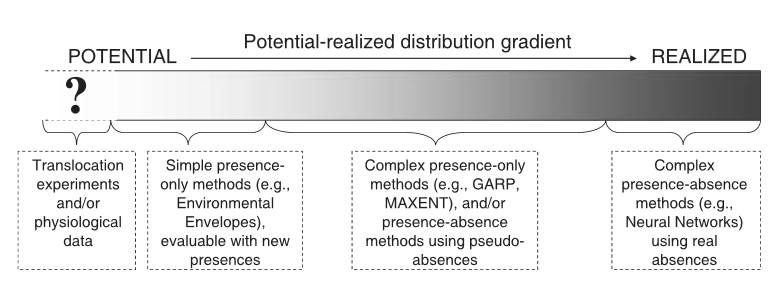
The following words are often used interchangeably when discussing a species distribution: habitat, environment, and niche. These words have been considered “plagued by loose and inconsistent applications of the concepts in describing different methodological approaches” and this paper implies that there is an overall confusion of what is actually being modeled. Generally, the concept of habitat in species distribution is described as being associated with descriptive/correlative analysis of the environments of the organisms and useful in statistical models of species distributions and abundances, while the niche concept is reserved for mechanistic analysis of how different environmental factors in an organism’s habitat interact with the organism itself.  While distributions can be potentially predicted by modelling descriptions or correlations between organisms and habitat components, it is suggested to model an organisms niche mechanistically to fully understand and explain distributional limits. This is particularly true when trying to predict an organism’s distribution under altering scenarios, such as climate change. ‘Environment’ would refer to the biotic and abiotic phenomena surrounding and potentially interaction with an organism. Two ways to model species distribution taking into account these “confusingly interchangeable words”, are to 1) use the correlative approach, distribution data and GIS habitat data are associated statistically, often in the form of a regression model then interpolated across regions for which spatial data is available to predict areas of high probability of occurrence (use of the habitat concept) and 2) the mechanistic approach (use of the niche concept) in which the interaction between the properties of the organism and the environmental conditions surrounding it are mechanistically modelled and mapped onto the landscape. Although this paper seems like basic definition issues, these words can often be interchangeably used across different published papers which could be confusing for readers who may be just grasping the ideas and concepts. Thus, this calls for more consistent and universal use of such words to avoid confusion and to pay more attention to the definition and the context.


Not as good as they seem: the importance of concepts in species distribution modelling

Alberto Jiménez-Valverde, Jorge M. Lobo and Joaquín Horta
Diversity and Distributions, (Diversity Distrib.) (2008) 14, 885–890
doi: 10.1111/j.1472-4642.2008.00496.x

Three important concepts must be kept in mind when modelling species distribution: 1. The distinction between potential and realized distribution 2. The effect of the relative occurrence area of the species on the results of the evaluation of model performance and 3. The general inaccuracy of the predictions of the realized distribution provided by species distribution modelling methods. This paper mentions that different distribution modeling techniques should be used depending on whether the purpose is to determine potential vs realized distribution (Figure 1). Based on previous literature on a variety of species distribution models, the authors ask whether complex models tend to be more accurate then simpler techniques and this question comes into effect when considering a species potential vs. realized distribution (because realized is more context dependent and may require higher resolution data and therefore more complex). Sometimes when determining potential vs. realized distribution, different types of data, such as absence in addition to presence data will be needed, which can help to infer species exclusion because of an interaction with another species. It is also suspected that rarer species models are more accurate because presence data has more specific environmental associations. Thus, data type can also influence whether one thinks that complex provides better results that simpler models. Another issue can arise with the evaluation of model performance which can be biased towards a better performance of complex techniques due to their potential to overfit models of the training data. The performance of the models should be evaluated by examining errors of omission and commission separately and by taking into account the ratio between the extent of occurrence and the whole extent of the region of study. Overall, understanding which models to use requires a clear understanding of the question at hand and the type of data available/feasible to collect in addition to the species biology.

Fig. 1. An overview of suggested models depending on whether potential or realized species distribution is desired.

Capture

Drought sensitivity shapes species distribution patterns in tropical forests

Engelbrecht, BJ, Comita, LS, Condit, R, Kursar, TA, Tyree, MT, Turner, BL, & Hubbell, SP 2007, ‘Drought sensitivity shapes species distribution patterns in tropical forests’, Nature, vol. 447, no. 7140, pp. 80-82

DOI: 10.1038/nature05747

Investigation into the mechanisms behind tree species distribution along an environmental gradient. Differential drought sensitivity shapes plant distribution in tropical forests at both regional and local scales. 48 species were evaluated on their local and regional distribution within a network of122 inventory sites spanning a rainfall gradient along central Panama. The results suggest that niche differentiation with respect to soil water availability is a direct determinant of both local and regional scale distribution of tropical trees. However, global climate change and forest fragmentation can alter soil moisture availability, causing a change in tree species distribution which will be important to monitor for future studies. Regional species distribution – presence/absence and density of species were collected from sampling plots that were situated on both the wet (Caribbean) and dry (Pacific) sides of the Isthmus of Panama. An index of dry season response for 44 of the species was based on the fitted probability of occurrence toward the dry end and toward the wet end of the gradient. Drought sensitivity was a significant predictor of the probability of occurrence of the species on the dry relative to the wet side. At the local scale – species density was collected from sampling plots on wet and dry slopes within Barro Colorado Island. Local associations were analyzed of the tree species with dry and wet habitats. The paper further addresses interactions between environmental conditions that may or may not indirectly influence drought resistance (i.e. water availability) which is suspected to be a major driver of tree species distribution. Linear regressions were used to examine whether species reactions to drought or light were significant predictors of their densities in dry vs. wet sites. Knowledge of these more specific influential factors can help predict what impacts climate change and deforestation can have on future distributions of the species. Instead of using linear regression to detect significant predictor variables and this way determine species distribution, this project could have also benefitted from using a machine-learning algorithm of an ecological niche model. Because all of the elements were available, such as species presence/absence and environmental data it would have been interesting to compare their results with an ENM and determine which methods works best.

Geographic distribution and ecology of potential malaria vectors in the Republic of Korea.

Foley DH, Klein TA, Kim HC, Sames WJ, Wilkerson RC, Rueda LM. J Med Entomol. 2009, 46: 680-692. DOI: 10.1603/033.046.0336

Larval and adult mosquito collection data were used to develop ecological niche models for the potential geographic distribution for eight anopheline species in the Republic of Korea with the intention to compare species distribution of the mosquitos to areas of suspected malaria transmission in order to understand current and potential malaria risk and determine whether there is a particular species that has been responsible for malaria resurgence. Ecological requirements for each species were studied using occurrence only data. Mosquito occurrences that had between 9 and 106 points were used, however, to avoid spatial autocorrelation and ensure data independence, localities that were at least 5km apart were used. Environmental data was downloaded from the WorldClim dataset, which included monthly temperature, precipitation, and the 19 “bioclimatic layers”. Topographic, historic (?) land use, and NDVI layers were also used.  Both GARP and MaxEnt were used to develop the ENM because they have both been used in previous mosquito distribution models and overall have been well received. Garp utilizes the iterative process of rule selection, evaluation, testing, and incorporation or rejection with the intent to “evolve” to maximize predictive accuracy, while MaxEnt also uses testing and training data with a decision threshold to determine presence or absence of a species given the environmental data layers. Prediction success of the distribution models were better than random except for Garp models for 2 mosquito species and MaxEnt for one mosquito species. Reasons for poor distribution prediction may have stemmed from spatial resolution that is too coarse and does not match up with some mosquito species smaller scale environmental needs. Fitting species distribution with records of malaria outbreaks suggested that all species occurred where malaria outbreaks occurred, but some species occurred less frequently. Furthermore, the models were able to determine which environmental variables or landscape characteristics are considered more influential on the distribution of a species. Although these models proved useful in determining geographic distribution across large scales, it could be improved by using absence data as well (instead of presence only), more spatially separated data (instead of data ‘clumped’ around certain locations, higher resolution environmental data that is more up-to-date and land use data (to find whether certain types of disturbance may be associated with a greater abundance of a certain type of mosquito?). Also, another way to improve these models would be to incorporate some kind of interaction variable between species, especially during larval stages.

Fine-Scale Predictions of Distributions of Chagas Disease Vectors in the State of Guanajuato, Mexico

, , , , , , , ,

http://dx.doi.org/10.1093/jmedent/42.6.1068

Many species distribution models (specifically regarding models for the triatomine vector) are conducted at large geographical scales whereas smaller local scales may be more useful in understanding significant drivers of specific triatomine species distributions and thus a more localized disease risk. Lopez-Cardenas assesses a fine-scale distribution (“ a landscape view”) for 5 triatomine species: Triatoma Mexicana, T. longipennis, T. pallidipennis, T. berberi, and T. dimiata by geo-referencing collection localities and using ecological niche modeling with an evolutionary-computing approach. Triatomine species were collected from the field from 201 communities within Mexico. Risk for disease transmission was also assessed from niche mapping results. Predictor variables included the use of multi-temporal, remotely sensed environmental data sets as surrogate for climate data which permits fine-scale predictions across landscapes since climatic monitoring stations are too sparse to permit development of fine-scale climatic maps. Triatomine occurrence points, were used for each triatomine species and processed in the model GARP to determine species ecological niche.  Data were separated into training and testing data and rule variable selection was developed through an iterative selection process. 100 models were generated from the same selective process and the best models were chosen based on ideal omission and commission errors. Chi-squared test was used to compare observed success in predicting distributions of test points with those expected under random models. Results from using GARP has suggested which species provide a greater risk to human health based on their distribution patterns in Mexico. In retrospect, the quality of data they collected seemed ideal for any vector-presence study I’m just curious why they would use occurrence only models such as GARP when they have a good idea of species absence data as well. Perhaps it would be better to use presence-absence models in this situation because of the quality and credibility of their data, and therefore are more likely to have true absences.


The impact of climate change on the geographic distribution of two vectors of Chagas disease: implications for the force of infection.

Medone, Paula, et al. “The impact of climate change on the geographical distribution of two vectors of Chagas disease: implications for the force of infection.” Phil. Trans. R. Soc. B 370.1665 (2015): 20130560.

Rabinovich et al 2015 models the climatic niche distribution of two Chagas disease vectors, Rhodnius prolixus and Triatoma infestans, in Venezuala and Argentina, respectively. ENM were used to determine the current distribution and potential future distribution under climate change scenario using WorldClim environmental data set, determine which variables are significant drivers of triatomine distribution and evaluate potential disease risk shifts in areas known to have high disease prevalence. The authors used presence-only data of the two triatomine species generated from range maps (which may have contained pseudo-absences). To prevent over-fitting of the niche models, 5% of the data were randomly selected for presence points of each species from the complete distribution range. MaxEnt was used to predict the climatic niche for both species under current and future conditions and partial area under the curve (pAUC) was use to evaluate the goodness-of-fit for the models predictions. An interesting follow up would be to understand why AUC has been criticized and pAUC considered favorable (since this was the first time I had heard of pAUC). To evaluate transmission risks to humans and climate suitability, two approaches were used: 1) directly relating suitability and the rate of acquiring the disease (force of infection, FOI) for specific regions in the countries and 2) relating suitability with household vector density and then vector density with FOI. The two approaches likely come with a slew of assumptions such as population demographics associated with infection risk from rural villages and also rely heavily on health data that may be biased or erroneous (since this is considered a neglected disease). However, there probably is no alternative. Results suggest that climate change will have a different impact on each triatomine distribution and transmission risk, which depends on the biology of the triatomine, although a general decrease in disease risk associated with 2050 climate conditions was the take home message. Although the papers methods and approach were useful, it seemed too general to make any solid conclusions from and instead of answering questions, it creates more regarding which (environmental, climatic, microhabitat, etc.) factors are actually important in the distribution of triatomines and how we can gather that data and how use that data for future projects.

Geographic distribution of Chagas disease vectors in Brazil based on ecological niche modeling.

Gurgel-Gonçalves, Rodrigo, et al. “Geographic distribution of Chagas disease vectors in Brazil based on ecological niche modeling.” Journal of tropical medicine 2012 (2012)

http://dx.doi.org/10.1155/2012/705326

Despite the efforts of domestic triatomine vector eradication, Chagas disease transmission in humans still poses a risk in Latin American countries. Determining risk in areas where sampling and data are insufficient or non-existent Gurgel Gonclaves et al, have turned to ENM to determine areas of risk that have been subject to poor sampling of triatomines with synanthropic tendencies resulting in low data resolution in Brazil. ENM was applied here to explore both geographic and ecological phenomena based on known occurrences of various species. They used 3563 records of occurrences within Brazil in which at least 20 unique occurrence points were chosen for 62 species (leaving only 17 to conduct ENM on). These points were analyzed with environmental data set NDVI and 19 bioclimatic WorldClim variables (conventionally used layers). MaxEnt was chosen due to the nature of the study at hand; because no extrapolation would be involved to apply or speculate distributions from other locations. Models from each species were then combined to overlay an area of risk within Brazil. To provide a view of species responses to environmental variation across Brazil, they plotted 1000 random points across the country and determined: 1. presence/absence of each species and 2. The values of the first two principal components of the bioclimatic data set. MaxEnt allowed them to determine that some triatomine species occur within specific biomes, while others are more generally occurring. They were able to detect biome association with specific triatomine occurrence. Determining high risk areas was one of the main objective for this paper, however because triatomines exist through Brazil, determining high risk areas could easily have been just the locations of rural villages. Other than using that reason to conduct the ENM, it otherwise seemed most useful when determining which environmental characteristics drive species distribution at the geographic level. Furthermore, have limited data on 62 species and only being able to conduct ENM on 17 species shows that the amount and type of data is very crucial and so this method is not very useful in studying rare or elusive triatomine species, which would overall be more interesting and probably most important.

Forecasting Chikungunya spread in the Americas via data-driven empirical approaches

Escobar et al. Forecasting Chikungunya spread in the Americas via data-driven empirical approaches. Parasit Vectors. 2016; 9: 112. Published online 2016 Feb 29. doi:  10.1186/s13071-016-1403-y

Chikungunya  is endemic to Africa and Asia and is transmitted  primarily by Aedes aegypti and Aedes albopictus. The authors map disease risk of the Americas using novel computational tools and data streams: weekly CHIKV reports, air travel, geographic distance and connectivity, and climate suitability of vector species. Using these data sources, the authors quantified imported cases, local cases at the country level, and geographic hotspots.

The geographic transmission hotspots were identified used SDM where transmission is limited by climate. The fundamental ecological niche was estimated using a climate envelope, based on minimum-volume ellipsoid describing ecological features of the occupied range. The number of WorldClim variables were reduced by used the top three components of a PCA instead of all variables. The niche centroid of the 3 components was then used to quantify proximity to centroid on a continuous map. Summary metrics were calculated for each country.

CHIKV was introduced to the Americas in regions with highly competent vectors. Identified hot spots for A. aegypti are Haiti, Dominican Republic, Puerto Rico, Guadeloupe, Dominica, Martinique, St Lucia, Saint Vincent and the Grenadines, and Grenada, plus on the mainland in coastal Venezuela and Brazil, across Central America, and in the lowlands of Peru and Bolivia. While Ae. albopictus had high areas of transmission in southeastern United States, southern Brazil, central Chile, Central America, and across the Andes Mountains in Bolivia.

Eight (and a half) deadly sins of spatial analysis

Hawkins, B. A. (2012), Eight (and a half) deadly sins of spatial analysis. Journal of Biogeography, 39: 1–9. doi: 10.1111/j.1365-2699.2011.02637.x 


Spatial autocorrelation is not the only issue of spatial analysis. Additionally, this autocorrelation is not just a data quality issue. Issues raised are focused on regression models.

1. Spatial autocorrelation generates bias
Nature is autocorrelated, species are distributed non-randomly. Understanding the pattern in autocorrelation the goal of ecology and biogeographers. However, statistical parametric modeling often requires random data- so perhaps this approach, specifically significance testing, is not appropriate.

2. Spatial regression is best
A common assertion in the literature: If ordinary least square regression is biased, then generalized least square must be the best (and only) method.
But there are multiple ways to to cope with the bias (or uncertainty), there is no single best approach. Alternatives include presenting multiple models or model averaging, however, this will never correct for uncritical use of multiple regression.

3. The world is stationary
Stationarity is the assumption that predictor/response variables are invariant throughout data. The consequences of this violation varies with model choice- but will influence the interpretation of parameter values. Despite non-stationarity being common in ecological data, very few studies test or account for this assumption. This needs to be done at the very least, if ideally the authors do not incorporate non-parametric methods such as CART.

4. Partial regression coefficients mean something
Ecologists would like to identify the most important influence on spatial patterns, but multiple regression is designed to ignore correlations among predictors making this a very poor approach. Alternatives, such as, CART or SEM are better suited to assert causal links.

5. Regression coefficients identify effects
`Correlation is not causation’ is well known, and ignored. The distinction between statistical effect and mechanistic effect need to be clearer in both communication and thought.

6. Species richness generates bias
This is a misunderstanding of sampling theory. All samples will converge to the parametric mean, if the sample is random. The non-random assortment of species are the patterns we are trying to test. The need to correct for species richness is the result of confusion between bias and precision. It is clear that the claim that richness generates bias in estimates of means is without foundation.

7. The earth is round (P<0.05)
P-values and AIC/BIC are not complementary tests for model evaluation. Either the model should be compared to the null (as in p-value) or the most parsimonious model should be chosen (AIC/BIC). CART can lend itself to model selection based on information theory.

8. Spatial processes explain spatial patterns

Legendre (1993) provided a heuristic method for distinguish- ing environmental and spatial structure in ecological data by means of a partial regression (or constrained ordinations) that partitions ‘(a) nonspatial environmental variation’, ‘(b) spa- tially structured environmental variation’ and ‘(c) spatial variation of the target variable(s) that is not shared by the environmental variables’ (p. 1666). His use of the language was careful, and this method is now widely used, but it is not uncommon to read that (c) is the effect of pure space, or the effect of spatial processes. Is it?

8 and half. Spatial autocorrelation causes red shifts in regression models

Overemphasize on the importance of broad scale (vs local) predictors is called a red shift. If anything, we have this backwards. Range maps contain false positives, and survey data contain false negatives. Range maps are created by filling in ‘presences’ between points, meaning that closer cells will have more distortion than distant cells. Of course, the level of distortion is grain dependent, but so are the processes that influence diversity.

Can changes in the distributions of resident birds in China over the past 50 years be attributed to climate change?

Among vertebrates, birds may be the most sensitive to climate change.  Over the past 100 years, the global mean air temperature has increased by 0.85°C. In the last decade, this shift in temperature has been accompanied by a northern shift of bird species in China. The author’s use species distribution models to ask if the rising temperature caused the changes in 9 resident bird species (20 subspecies)  range over the last 50 years.

The 9 chosen species are endangered in China and have a large point distribution data set, additionally these birds have been found outside of the historical boundaries in recent years. Given that the dataset consists of presence-only data and uncertainty in the biotic and abiotic variables, the authors used a fuzzy envelope model trained on data from 1951-1960. Climate factors were chosen based on there influence on environmental suitability for reproduction. From this the suitability for each grid cell for each year between 1961-2010 was calculated. The total suitability for each grid was calculated by summing the suitability across the years. The model accuracy was evaluated using kappa-statistic (k) using the 1951-1960 as baseline for each decade. 

Wu_fig7

The range centers of 7 species shifted northern, 6 species east, and 3 species west ward. The suitable range of 9 subspecies increased with climate changes, while others exhibited no change.