Christina Varian – Page 2 – ECOL 8910: Perspectives in Computational Ecology

On estimating probability of presence from use–availability or presence–background data.

Phillips, S. J. and Elith, J. (2013), On estimating probability of presence from use–availability or presence–background data. Ecology, 94: 1409–1419. doi:10.1890/12-1520.1

The paper investigates statistical methods (specifically logistic models) that estimates the probability that a species is present at a site conditional on environmental covariates and further addresses the disagreement in the literature on whether probability of presence is identifiable from presence-background data alone. The probability of presence is identifiable if one makes strong assumptions about the structure of the species probability of presence, however some view the assumptions unrealistic and the risk of deviating from strong assumptions can result in poorly calibrated models. An experiment (outlined below) also demonstrates that an estimate of prevalence is necessary for identifying the probability of presence. It is suggested that presence-background data must be augmented with an additional datum to reliably estimate absolute probability of presence. Methods: Seven simulated species whose probability of presence is defined by the seven functions: constant, linear, quadratic, Gaussian, Semi-Logistic, Logistic 1 and Logistic 2 (whose probabilities were bounded by 0 and 1) – which represent a variety of shapes of the response of a species to its environment – were used, in addition to randomly drawn data with 1000 presence samples and 10000 background samples chosen uniformly (0 to 1). Data was used with 5 maximum-likelihood-based methods (abbreviated as EM, SC, SB, L1 and LK) for deriving logistic models from presence-background data. Method inputs varied by 1) using a strong parametric assumption to make probability of presence identifiable (which the output failed to estimate the species probability because it fails to acknowledge species response to environment as identified in L1 and LK) and 2) requires the user to supply an estimate of the species population prevalence (as in EM, SC, SB, which was ultimately recommended to use). Based on the papers results, there is no alternative to collecting quality field work data (as opposed to making strong assumptions as in (1)) which further points out the importance to address the complexities in species-environment relationships. I thought it was pretty obvious that one cannot make strong assumptions when determining a species presence, although it might be easier for the sake of using models, but when you take an ecologist (or more specifically a wildlife manager) point-of-view determining what information goes into a model is probably more relevant.

Historically calibrated predictions of butterfly species’ range shift using global change as a pseudo-experiment

Kharouba, Heather M., Adam C. Algar, and Jeremy T. Kerr. “Historically calibrated predictions of butterfly species’ range shift using global change as a pseudo-experiment.” Ecology 90.8 (2009): 2213-2222.

DOI: 10.1890/08-1304.1

Case study conducted by Kharouba et. al. used a climate and land use change scenario in Canada for a pseudo experiment to test model reliability for predicting species range shifts over long time periods (30-60 years) and very large geographical areas for 297 butterfly species. They used historical distribution data with six environmental predictor variables over a 10 million km2 range and modeled with MaxEnt. Steps included: generating a historic species distribution model (1900-1930), projecting these models with environmental data from 1960-1990 (projected model), model species distribution using current environmental data and species occurrence records (current model), and test the ability of using projected models to predict the current models (by comparing actual current distribution) and determine whether this method is suitable to predict species distribution change over time. The accuracy of each model was determined using AUC. Models that constructed historic and current species distribution individually had high value AUC, but when historic model was used to project current distribution, it both underestimated and overestimated suitable habitat when actually compared to the current distribution. Results depended on the species of interest and how that species responds to environmental change. Using this method to predict future distribution in response to climate change can be considered reliable, but projection accuracy depends on scale (pixel vs. region). Other factors to be considered when using this method of modeling, or could make this method even stronger, should include plant responses (butterfly resources) to climate change, feeding habits of the butterfly (i.e. generalist vs. specialist butterflies), species traits and their responses to climate change, and species response to community-level changes.

The ability of climate envelope models to predict the effect of climate change on species distributions

Hijmans, Robert J., and Catherine H. Graham. “The ability of climate envelope models to predict the effect of climate change on species distributions.” Global change biology 12.12 (2006): 2272-2281.

DOI: 10.1111/j.1365-2486.2006.01256.x

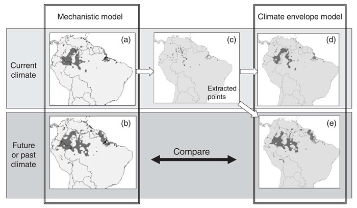
Hijman and Grahams objective was to evaluate whether Climate Envelope Models (CEM) are as successful in predicting species distribution under future climate change scenarios as it is in predicting current species distribution. They evaluated CEM ability by comparing CEM predictions with predictions obtained from Mechanistic Models (MM, which are based on an understanding of species physiology while CEMs use known geographic locations of a species to infer on their environmental requirements). They evaluated data from 100 plant species for past, current, and future distributions, by comparing MM results with four different CEM that covered a range of statistical approaches: BioClim, Domain, GAM, and Maxent and used range size, overlap index, false positive rate, and false negative rate to determine how well species distribution with CEM corresponds with MM (Generally illustrated in Fig. 1). The concern is that some CEMs may be unsuitable to predict species ranges under future climate because 1) cannot be tested using independent model training and testing data sets (i.e. no observed data for future scenarios and 2) a statistical model in which the inferred environmental requirements may not be suitable for truly classifying suitable vs. unsuitable environments. Hijmans suggests to compare results from CEM with MM, because using MM will model species distribution using physiology independent of climate. However, the only problem with MM is that physiology data is not always easy to gather. There was considerable variation between CEM and ability to reproduce the predictions from MM. Maxent and GAM provided good estimates for range shift with climate change. Domain underestimated range size. Bioclim underestimates future ranges, so would be considered a conservative approach, for example for reserve planning. Don’t even go with Domain, because it was considered too sensitive to the number of environmental variables used to predict species distribution. They came to the conclusion that some CEMs are reasonably good at predicting species dristributions under a climate change scenario.

In this paper, to assess species distribution changes in response to climate change, nonclimatic effects were eliminated. This is not very realistic however, because species distributions is likely influenced by both biotic and abiotic factors. It would be interesting to take biotic factors into account, because most likely species interactions with one another may be indirectly linked to changes in distribution driven by abiotic factors (one would persist and the other may not?). Also, applying this to vertebrate data, and even more interestingly, a migrating species, would be a great next step for using CEM to predict future species distribution.

(Figure caption: Approach used to evaluate the ability of climate envelope models to predict species distributions under different climates. A mechanistic model is used to predict the potential distribution for a species under current (a) and future (or past) (b) conditions (light gray = not suitable, dark gray = suitable). Points are extracted randomly from the area deemed currently suitable for the species (c). These points are used in the climate envelope model for current (d) and future (e) conditions. The statistical model is evaluated through a comparison of (b) and (e).)

Model‐based uncertainty in species range prediction

Pearson, Richard G., Wilfried Thuiller, Miguel B. Araújo, Enrique Martinez‐Meyer, Lluís Brotons, Colin McClean, Lera Miles, Pedro Segurado, Terence P. Dawson, and David C. Lees.
Journal of Biogeography 33, no. 10 (2006): 1704-1711. doi:10.1111/j.1365-2699.2006.01460.x

This paper overall addresses the source of uncertainty in assessments of the impacts of climate change on biodiversity. Pearson et al. used a variety of environmental niche modelling techniques (artificial neural network, climate envelope range, constrained Gower metric, classification tree analysis, genetic algorithm, generalized additive model, genetic algorithm for rule-set prediction, and generalized linear model) to evaluate the impact (magnitude of variation) of model choice on predicted species distribution under current and predicted climate change scenarios and why model outputs may differ. They used data on four endemic plant species of Protoeacea found in S. Africa collected from 3996 sampled sites located within different 1’X1’ cells and used identical input variables that are considered critical to plant physiology and survival. Model predictions were compared by testing agreement between observed and simulated distributions for present day (using AUC and kappa statistics) and assessed consistency in prediction of range size changes under future climate using cluster analysis. Distribution was characterized by the number of grid cells occupied. Technique was applied to 70% randomly selected sites and 30% was used to test agreement between observed and modelled distributions. Under climate change scenarios, for all models, except CER and GA, the suitability for each cell was calculated at decision thresholds increasing from 0-1 and used cluster analysis to group predicted ranges from different methods under current and future climate conditions. They found that: variation between model predictions can be attributed to models that use presence-only data vs. presence-absence data (so realized vs. fundamental niche predictions) as they had performed differently. Another key factor that should be carefully considered for ENMs is model extrapolation assumptions. For example, instances of extrapolating environmental variables under climate change range expansion yielded uncertainty in model predictions. Similar to class discussion this week, this paper presents models on an endemic (and plant) species, it would be interesting to apply the same objective to a non-endemic vertebrate species and compare model predictions.

Sensitivity of predictive species distribution models to change in grain size

When using species distribution models, grain (resolution) size is a spatial factor that may influence predictive model outcomes. Guisan et. al. (2007) tested the effect of grain size on SDM by comparing model performance of 10 predictive modelling techniques (DIVA-GIS, DOMAIN, GLM, GAM, BRUTO, MARS, BRT, OM-GARP, GDMSS, and MAXENT-T) on presence only data of 50 species in 5 different regions (from Elith et al 2006) and also determined whether affects observed were dependent on the type of region, modelling technique, or organism considered. Model performance at two grain sizes (original and 10-fold) was assessed and prediction success was compared and ranked using Area under ROC curve. Increasing grain size did not affect model performance however it did degrade models on average. Although surprised by the outcome, the somewhat fundamental question reflects realistic issues in SDM. The testing 10 modelling techniques was a well thought out approach to determining factors that apparently aren’t influenced by grain (unless original data lacked predictive power that wouldn’t be influenced by scale anyway). It would be interesting for a follow up paper to test other variables that may be more affected by changes in grain size (sessile organism, species with small home ranges, or factors at the microhabitat level).