Big Data, new epistemologies and paradigm shifts

Kitchin, R., 2014. Big Data, new epistemologies and paradigm shifts. Big Data & Society, 1(1), p.2053951714528481.

This article argues that the explosion in the production of Big Data and the advent of new science epistemologies where questions are born from the data rather than testing a theory by analyzing data has far-reaching consequences to how research is conducted. One section evaluates whether the scientific method is rendered obsolete with the production of Big Data. Instead of making educated guesses about systems, constructing hypotheses and models, and testing them with data-based experiments, scientists can now find patterns in data without any mechanistic explanation at all. But in some fields, this doesn’t really matter. For example, in online retail stores Person A might be known to like item A and most people that like item A also like item B. In this situation, the mechanism does not really matter for the retail company to sell more items. Thus, mining the entire population’s behavior for prediction trumps explanation for the retail markets. But the result is an analysis that ignores important effects of culture, politics, policy, etc. So expanding these ideas to the field of biology might include a bioinformatist that view the complexity of biology in a much different way that an experimental molecular biologist. To an informatist, data can be interpreted free of context and domain-specific expertise but it might be low on logical interpretation.

The evolution of science through four broad paradigms based on the method of data collection

It seems to me that the majority of ecologists are aware of the concerns that Kitchin raises and would probably side with him on most points, especially when thinking about mechanisms causing patterns rather than settling with knowing the correlations that coincide with them. Nevertheless, I think it was a good read and one that helped me contextualize some disagreements between Big Data and production of new science.

A climate of uncertainty: accounting for error in climate variables for species distribution models

Stoklosa, J. et al., 2015. A climate of uncertainty: accounting for error in climate variables for species distribution models R. B. O’Hara, ed. Methods in Ecology and Evolution, 6(4), pp.412–423.

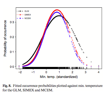
An important consequence of biased parameter estimates is biased projections under changes of environmental variables. There is a large distinction between GLM and the errors- in-variables models.

Climate variables used in species distribution models are estimates of true spatial climate and are therefore subject to uncertainty. The uncertainty itself can have spatial structure, further complicating consistency of estimates. The authors of this study chose to use PRISM (parameter elevation relationships on independent slopes models) to obtain estimates of climate uncertainty. To do this, they construct grids of approximately 800x800m size and use these estimates as an upper bound to prediction error variance of the climate model.

They also wanted to understand what happens if this uncertainty is ignored. Other fields, such as engineering and medicine, use measurement error models that allow uncertainty in explanatory variables (errors-in-variable) but can sometimes lead to biased estimates. This study used hierarchical modeling and simulation extrapolation to account for errors in explanatory variables. Wren presence/absence data (n=1048 data points) was obtained from birders at several points along a transect of the Eastern US. They test these methods on the Carolina wren in the US and on simulated species to look at how well GLMs predict and project to new scenarios when prediction error is ignored versus when it is accounted for. The main effect of ignoring uncertainty in climate variables was an increase in bias and a decrease in power as the error increases. These methods seem likely to be useful in situations where a species is patchily distributed or in environments that are spatially autocorrelated.

Contemporary white-band disease in Caribbean corals driven by climate change

Randall, C.J. & van Woesik, R., 2015. Contemporary white-band disease in Caribbean corals driven by climate change. Nature Climate Change, 5(4), pp.375–379. linkScreen Shot 2016-04-22 at 4.21.25 PM

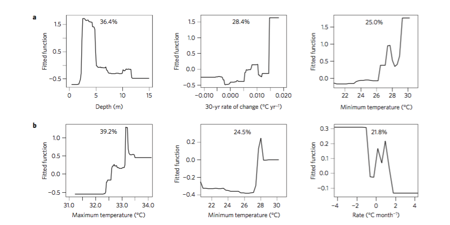
Populations of two dominant coral species, Acropora palmata and Acropora cervicornis, have declined more than 90% in the past 40 years. This decline is mostly attributed to white-band disease. Although other coral diseases have been linked to increases in sea surface temperature (SST), there is no definitive evidence for this in white band disease. To understand the response of white band disease to climate change related variables, the authors used boosted regression trees (BRTs), with presence and absence of disease data in a total of 473 coral colonies from 1997 to 2004. Stochasticity was incorporated into their models by bagging to fit each new tree and a k-fold cross-validation was used to train (90%) and test (10%) each model. The relative contribution of each predictor variable was estimated, and any interactions between predictor and variables were examined. Their models performed well for both species, with AUCs of 0.85 and 0.72. For both species, a rise in minimum SST seemed to play a role in the increase in white-band disease. For one of the species, the rate of increase in SST over the past 30 years showed a steep rise in relative contribution to prediction of white band disease after about 0.015 degrees C per year. Since global models predict a mean increase in SST of .027 C per year from 1990 to 2090, many reefs currently without white-band are likely to have disease in the future.

Eight (and a half) deadly sins of spatial analysis

Hawkins, B.A., 2012. Eight (and a half) deadly sins of spatial analysis. Journal of Biogeography, 39(1), pp.1–9.

Hawkins argues that many ecologists are of the understanding that the existence of spatial autocorrelation is a bias or artifact of sampling that must be removed rather than embraced when trying to model their distribution. In this opinion essay, he argues against this notion as well as against eight (and a half) other commonly held perceptions in ecology. First, spatial autocorrelation is not bias. Instead this autocorrelation in nature is what we wish to understand. Indeed, spatial autocorrelation in nature is separate from residuals in a model. Second, spatial regression is not always the best according to Hawkins and some statisticians. In the Beale (2010) paper that we read, we did see that OLS produced estimates that were not all that different from spatial models and here, Hawkins notes that even when studies find that spatially explicit model are best arise in simulation studies of species rather than using real data. Thus, muddying the waters for making generalized claims about how spatial models are always better. Third is the assumption of stationarity among the entire landscape. Authors often fail to report whether or not they have determined whether their data abides by this assumption. Fourth, Hawkins argues that partial regression coefficients are not very meaningful for these contexts. The main idea of this section is just that we can’t quibble over which particular type of multiple regression, and values of coefficients, is the best method for understanding a process. Fifth, was correlation does not equal causation and argues that although many ecologists have heard this mantra, some still don’t uphold the value of the statements. Sixth was the idea that species richness causes bias. Hawkins emphasizes that if the species is prevalent in an area, we should not wish to remove this phenomenon from our data. Usually, he states, this type of misconception is due to a confusion of precision with bias. Next, he argues that spatial processes explain spatial patterns (i.e. there are biological processes operating in a spatially structured environment that we wish to understand). Finally, he notes that spatial autocorrelation causes red shifts in regression models. This means that there is an over-estimation of importance of broad scale predictors in OLS multiple regression models. He argues that this point is not important at all. Take away points from this paper include: (1) that we should not try too much to focus on methodology when describing species distributions. If we do this then we run the risk of trying to capture all complexity in our data rather than understanding it. (2) Many of the disagreements among researchers using multiple regression tools stem from the lack of understanding of the assumptions that these models make. Although I agree with his findings about understanding assumptions and autocorrelation for multiple regression models, I find it difficult to validate his opinions on all matters of these subjects because he lacks citations backing up his claims.

Inference from presence-only data; the ongoing controversy

Hastie, T. & Fithian, W., 2013. Inference from presence-only data; the ongoing controversy. Ecography, 36(8), pp.864–867.

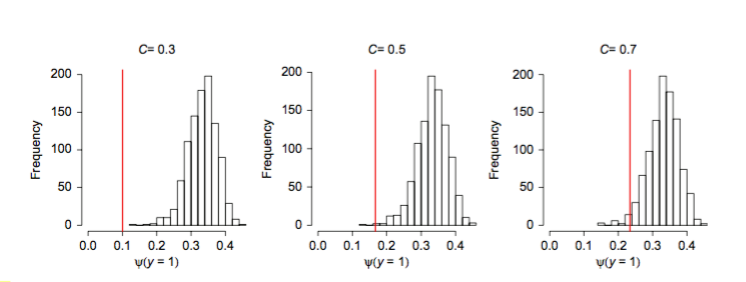
In response to Royle et al. (2012), Hastie & Fithian (2013) question whether it is possible to estimate the overall species occurrence probability, or prevalence, given presence only data. The main concern with Royle et al. (2012) is their assumption of parametric form for nearly log-linear variables. Problematically for most real world data, the functional forms are almost never linear. Royle et al. (2012) approach of linear approximation is a useful simplification that allows researchers to estimate prevalence. But Hastie & Fithian (2013) argue that these assumptions are too arbitrary to be robust in practical settings. However, by assuming this, MLE methods can be used to estimate species probability of presence. To illustrate this point, they simulate nearly linearly logistic data and fit a linear logistic model using likelihood values to generate a large sample of values of x (geographic sites representing a unit of area), via the uniform distribution of sampling to determine presence/absence points. Next, they subset 1000 values of x’s, which had the species present. Figure 2, shows results from three separate simulation runs with the red line showing the true value for the species occurrence probability. In all cases, the values of the histogram bear no relationship to the true values of probability of presence. This paper clears up the main argument against using presence-only data to calculate the full support of species prevalence.

Point process models for presence‐only analysis

Renner, I.W. et al., 2015. Point process models for presence‐only analysis R. B. O’Hara, ed. Methods in Ecology and Evolution, 6(4), pp.366–379.

Renner et al. (2015) discuss the commonalities between MAXENT, PPMs, and regression for presence-only data. Using a data set on 230 presence-only locations of Eucalyptus sparsifolia in Australia, the authors highlight key ideas and benefits of PPM. A key idea in this paper was to explain PPMs as applying a regression method to point event data, and interpret the intensity (the number of presence records per unity area) as the target of interest. An important benefit of this PPM specification is that there is greater clarity around the issue of how to choose sampling points, and the possibility of querying the data being analyzed to verify that a given choice of sampling points is appropriate. In their example, they were able to show that the sampling points required for sufficient estimate convergence of the log-likelihood was closer to 100,000 that the commonly advocated 10,000 points. The reasoning for increased sampling under random sampling, as compared with survey sampling, is that it is more difficult to quantify uncertainty in the data. The authors caution that when constructing PPMs it becomes very important that you interpret what is being modeled appropriately. In particular, are you modeling intensity of sampled sites? Or intensity of individuals across a landscape? Do duplicate records exist? The authors make their data accessible from bionet.nsw.gov.au and DRYAD doi:10.5061/ dryad.985s5.

Potential for spread of the white-nose fungus (Pseudogymnoascus destructans) in the Americas: use of Maxent and NicheA to assure strict model transference

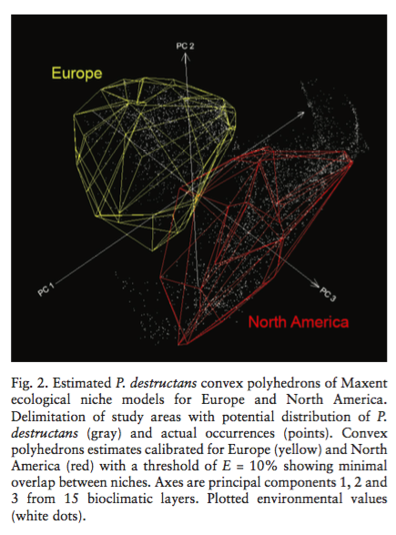
Escobar et al. (2014) model the range of Pseudogymnoascus destructans, the pathogenic fungus that causes white nose syndrome (WNS) in bats, in North America and Europe. They collected 218 observations of WNS for use in Maxent species distribution models. Variables in their model included the usual suspects (temperature, etc) along with some that are more important for modeling bat & fungus distribution (mean temperatures of coldest winters, annual precipitation, etc). Maxent models were then carried out on buffer areas of 500 km around European and North American occurrences. After calibration with Maxent of the training data in the two continents, projections of distributions to South America were generated. Three different approaches for projection were used: one without extrapolation, one with extrapolation, and NICHE-A models. NICHE-A models describe the fundamental niche in environmental space, thus identifying potential geographic places that may fall inside the minimum environmental ellipsoid containing all training points. In order to understand habitat differences in North America and Europe, the authors conducted tests for background similarity. They found that the two areas did not diverge significantly across the two continents, suggesting no real niche differentiation has demonstrably taken place between the two continents. However, depending on the projection approach and training data origin (from N America, Europe, or N America & Europe), Maxent transfer models differed markedly. Their use of NICHE-A, which reminds me of RangeBag, produced similar results to Maxent. I’m not sure I fully buy their results of projection to South America, given the differing community composition of bat species in South America and lack of clear evidence that WNS can infect these differing bat species. Even if these results give rise to error of commission in modeling WNS, I think the study is important because it can point ecologists and conservationists to regions at risk for transmission.


Escobar, L.E. et al., 2014. Potential for spread of the white-nose fungus (Pseudogymnoascus destructans) in the Americas: use of Maxent and NicheA to assure strict model transference. Geospatial Health, 9(1), pp.221–229. link to paperScreen Shot 2016-03-21 at 10.18.50 PM


Cross-validation of species distribution models: removing spatial sorting bias and calibration with a null model

Hijmans, R.J., 2012. Cross-validation of species distribution models: removing sorting bias and calibration with a null model. EcologyLink to paper

Spatial sampling biases, or the observation that testing presence points tend to be closer in space than do testing absence points (and the credibility of cross-validation for assessing model accuracy) remain large issues for SDMs. Hijmans (2012) evaluates two different ways of selecting testing-presence data and two ways of selecting testing-absence data in order to better understand how spatial sampling biases and cross-validation may lead to inflated confidence in SDMs. Indeed he found that a null model, based solely on distance to nearest presence point, performed just as well (.69) as Bioclim (.64) and Maxent (.73). This suggests that it can be difficult to directly interpret uncallibrated cross-validation results (as is seen in most studies using SDMs) and that calilibrating with a null model could lead to more accurate predictions. This study calls into question many results from SDMs, especially those using data that is inherently clumpy (e.g. museum records). I think this is an especially open area for research with questions such as: How can knowledge of a species biology be used to pre-process (filter) species occurrence data before being input into SDMs? Or how does clumpiness of species occurrence data affect predictability of species range?

Data prevalence matters when assessing species’ responses using data-driven species distribution models

Fukuda, S. & De Baets, B., 2016. Data prevalence matters when assessing species’ responses using data-driven species distribution models. Ecological Informatics, 32, pp.69–78.  link to paper

The accuracy of SDMs is highly dependent on the quality and quantity of data used such as size (i.e. the number of data points in a data set) and data prevalence (i.e. the proportion of presences in a data set) matter for SDM accuracy. Fukuda et al. (2016) investigated this observation by simulating nineteen sets of virtual species data in real habitat conditions (using field observations) and hypothetical habitat suitability curves under four conditions. Then they built SDMs in order to assess the effects of data prevalence on model accuracy and habitat information. The three SDMs they tested were the Fuzzy Habitat Suitability Model (FHSM), Random Forests (RF), and Support Vector Machines (SVMs). The effects of data prevalence on species distribution modeling were evaluated based on model accuracy (AUC & MSE) and habitat information such as species response curves. Data prevalence affected both model accuracy and the assessment of species’ response, with a stronger influence on species response curves. The effects of data prevalence on model accuracy were less pronounced in the case of RF and SVMs. Data prevalence also affected the shapes of the response curve where response curves obtained from a data set with higher prevalence were less dependent on unsuitable habitat conditions, emphasizing the importance of accounting for data prevalence in the assessment of species–environment relationships. Taken together, these results show that data prevalence should be controlled for when building SDMs.


Insights into the area under the receiver operating characteristic curve (AUC) as a discrimination measure in species distribution modeling

Jiménez Valverde, A., 2012. Insights into the area under the receiver operating characteristic curve (AUC) as a discrimination measure in species distribution modelling. Global Ecology and Biogeography, 21(4), pp.498–507. http://doi.wiley.com/10.1111/j.1466-8238.2011.00683.x

The AUC has been popularized as an omnipotent statistic in assessing the predictive accuracy of species distribution models. Most studies rationalize using the AUC value as a means to rank models by claiming that it avoids setting arbitrary thresholds for predictive decisions. Here, this claim is examined in relation to the relatedness between the AUC and sensitivity/specificity for modeling realized and potential niches. By definition, the AUC should not depend on any particular point on the ROC curve but in both simulated and real data there was a strong relationship between AUC values and certain points (the point closest to perfect detection and the point where specificity=sensitivity) on the ROC curve. In different settings (ie. studying the realized vs. potential niche), the fact that the AUC depends on certain points could be problematic because weighting errors should not be the same in each circumstance. For instance, type 1 errors (false positives) should not count as much as false negatives in modeling potential distributions as they do in modeling realized distributions. Thus, the author suggests that instead of reporting AUC values only, reporting contingency tables with varying thresholds for sensitivity and specificity may actually give us more insight into the predictability of SDMs. Overall, I agree with the author that researchers evaluating model performance need to be aware of the problems associated with using AUC values, but I am unsure of a systematic approach that would be appropriate to reporting contingency tables with thresholded values of sensitivity and specificity.