Tag: Robbie Richards

Anderson, Robert P., Daniel Lew, and A. Townsend Peterson. “Evaluating predictive models of species’ distributions: criteria for selecting optimal models.” Ecological modelling 162.3 (2003): 211-232.

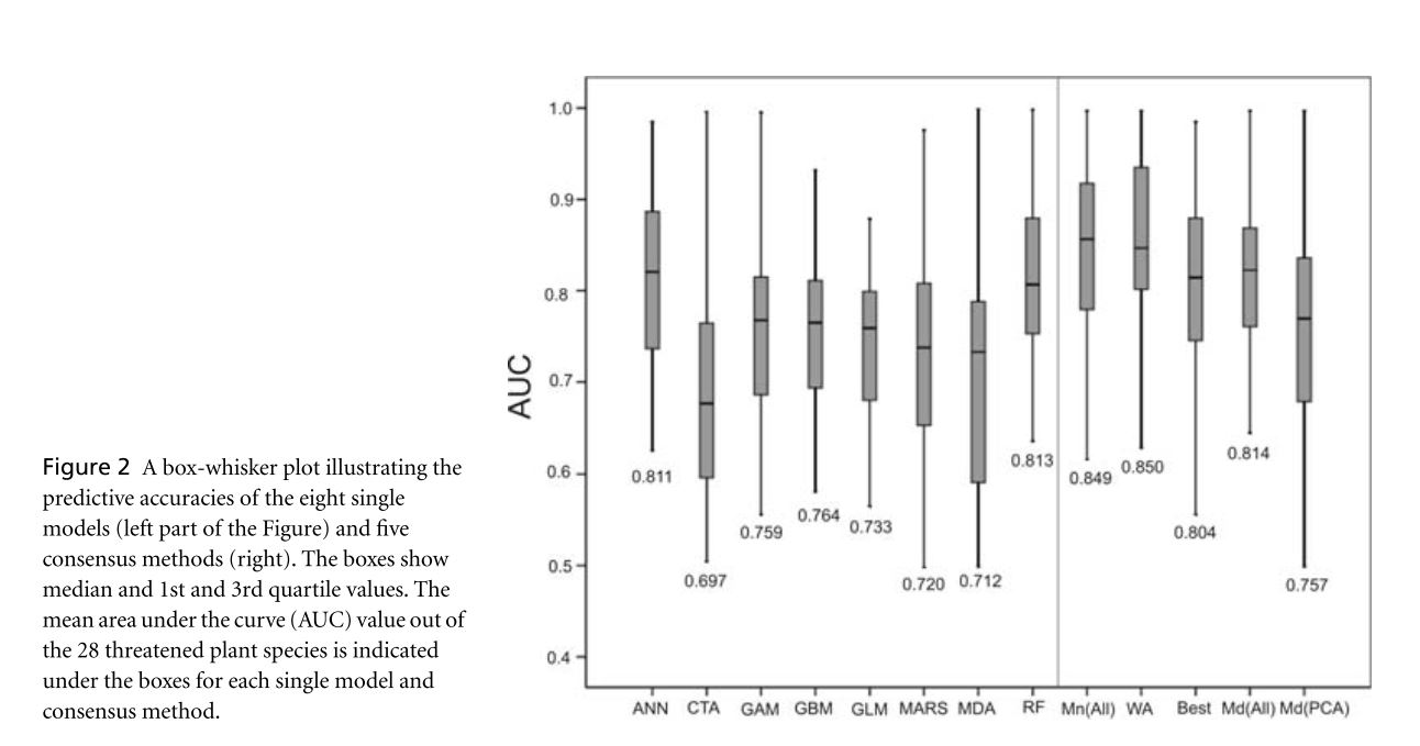
Anderson et al. assess the utility of consensus based predictors in species distribution models. These consensus predictors are made up of a number of fitted species distribution models of varying types. Component SDMs used for consensus modeling were GLM, GAM, MARS, ANN, GBM, RF, CTA, and MDA. These individual models were trained and evaluated on appropriate sub-subsets of the 70% training data subset in order to pre-evaluate these models for the purpose of consensus modeling. Consensus models assessed include Median(All) and Mean(All) which use the median and mean, respectively, of the predictions of all 8 models. The WA approach determines the 4 models with highest accuracy for a given species and computes a weighted average of their outputs. Median(PCA) is calculated as the median of the 4 models for which the variance of the predictions along the 1^st principle component of a PCA was the greatest. Finally, Best simply selects the best individual model based on the highest pre-evaluated AUC value. Each of these methods, as well of each of the individual models, were then evaluated using the 30% testing data subset. WA and Mean(All) provided significantly more robust predictions than all single models and all other consensus methods. WA was the best model with a mean AUC of .850 and better predictive performance than all single-models on 21 of 28 species. These methods provide a functional alternative to thorough single-model evaluation and comparison. The fact that the true consensus models consistently outperform the “Best” consensus model suggests the utility of these methods over comparative evaluation. These consensus models also effectively address the common issues that some single-models provide better predictions for interpolation and some for extrapolation and that the best evaluated model often varies significantly from species to species.

 

Václavík, T. and R. K. Meentemeyer (2009). “Invasive species distribution modeling (iSDM): Are absence data and dispersal constraints needed to predict actual distributions?” Ecological Modelling 220(23): 3248-3258.

http://www.sciencedirect.com/science/article/pii/S0304380009005742

Vaclavik and Meentemeyeer focus on the specific problem of modeling the distribution of an invasive species in the process of invading across a landscape. iSDM forces the modeler to address the likely generally common problem of dispersal limitations because there will necessarily be a number of locations across the landscape which are environmentally suitable but currently inaccessible to the species. This paper examines how the addition of a measure of dispersal to iSDMs will affect the performance of models, alongside an attempt to determine the differences in performance of models trained using presence-absence, presence-psuedoabsence, and presence-only data respectively. The authors perform this analysis using Phytophthora ramorum an invasive generalist pathogen responsible for sudden oak death. 890 field plots were exhaustively sampled for evidence of the pathogen in the summers of 2003, 2004, and 2005, providing a reliable presence-absence data set. A number of pseudoabsences, points randomly chosen that could potentially be inhabited by the pathogen but which were not sampled, equal to the number of verified absences was also generated. Eight environmental variables were used to fit models including a spatial distribution of the key infectious host of the pathogen. All models were trained either exclusively on these environmental variables or on these variables and a measurement of “force of invasion” at a given point. Force of invasion was modeled using the following equation:

where d_jk is the Euclidean distance between each potential source of invasion k and the target plot i. The parameter a determines the shape of the dispersal kernel where low values of a indicate high dispersal limitation, and can only be estimated from presence-absence data. For models trained without true absence data a simpler force of infection metric based exclusively on the above-mentioned Euclidean distances is used. Two models using just presence-only data (ENFA, and MaxEnt) and two using presence-absence or presence-pseudoabsence (GLM and CT) were used. GLM and CT based on presence-absence data, including dispersal constraints were the highest performing models. The inclusion of dispersal constraints significantly increased the performance of most models. Without dispersal constraints presence-only models outperformed the other types of models (though this phenomenon was clearly driven by the good performance of MaxEnt). Presence-only models generally predicted larger areas of invasion than both presence-absence and presence-pseudoabsence but all models showed a clear reduction in predicted area when dispersal constraints were included. This paper clearly illustrates the importance of including probability of dispersal into SDMs for species in the process of invading a landscape. The estimates of “force of dispersal” seem as if they would suffer substantially from any sort of bias in the sampling of presence points but they may have been able to account for this in their sampling strategy. It would be interesting and useful to determine how these concepts could be applied to non-invasive species which nonetheless have dispersal restrictions preventing them from accessing some favorable areas of a landscape, allowing us to generally relax the assumption of equilibrium of distribution across the landscape. Such applications would likely require a more complex estimation of force of dispersal. In these closer to equilibrium cases there are likely landscape features which significantly slow the rate of dispersal across certain areas, which in turn creates the pattern, so we cannot assume an even rate of dispersal over time and space.

 

Mod, H. K., et al. (2015). “Biotic interactions boost spatial models of species richness.” Ecography 38(9): 913-921.

Mod et al. attempt to address the general lack of quantitative consideration of biotic interactions in spatial modeling. Rather than basic spatial distribution modeling they model species richness across a landscape with two different methods. The first, somewhat familiar, method is stacked species distribution (SSDM) in which species distribution models are fitted for all species and then overlaid to determine species richness at each point. These models are fit using Generalized Linear Models (GLMs), Generalized Additive Models (GAMs), and Generalized Boosted Models (GBMs) and SSDMs are generally expected to overpredict species richness because the simple stacking implies no intrinsic environmental carrying capacity. They also use macroecological models (MEM) which directly model species richness and implicitly consider the environment to be limiting to the number of species. MEMs do not make any distinction between different species and generally tend to overpredict richness in species-poor sites while underpredicting richness in species rich-sites. In order to ascertain the ability of biotic variables to improve prediction and potentially correct these problems the authors build 3 different types of models and fit them to 3 taxonomic groups (vascular plants, bryophytes, and lichens). The first (Climate) model includes mean air temperature of the coldest quarter, growing degree days, and ratio of precipitation to evaporation, all broad-scale environmental drivers known to have a strong impact on vegetation. The second (Abiotic) model includes the Climate model as well as soil quality, soil wetness, and solar radiation as finer scale abiotic predictors. Finally the third (Biotic) model includes all previous predictors and the cover of three dominant species known to have impacts on the distribution of other species. These three species show both competition and facilitation based effects on a number of different species. In order to determine the fit of different models a linear regression was fitted to the plot of predicted vs. observed species richness (slope = 1 and intercept=0 represents perfect prediction). The inclusion of biotic variables increased fit and decreased bias for both methods across all taxa, the regression slope and intercept more closely approaching the ideal values. Mean AUC values averaged across all species models built for SSDM were higher as well. The fact that inclusion of biotic variables significantly improved fit across two different modeling methods strongly supports the extra explanatory/predictive power this data can offer. The widespread application of these methods relies, however, on the accurate determination of important biotic variables. This study was able to approximate competition pressure using the cover of 3 dominant species, an assumption which may be generalizable to a number of shade/nutrient limited plant systems. Systems with a more diverse and “evenly distributed” competition landscape may be very difficult to model in this way because knowledge of many species’ distributions across the landscape may be necessary to build these models.

Wharton, Trudi N., and Darren J. Kriticos. “The fundamental and realized niche of the Monterey Pine aphid, Essigella californica (Essig)(Hemiptera: Aphididae): implications for managing softwood plantations in Australia.” Diversity and Distributions 10.4 (2004): 253-262.

Wharton and Kriticos build two predictive models of the global distribution of the Monterey pine aphid Essigella californica. E. californica is native to western North America, from Southern Canada to Northern Mexico but has recently expanded to Europe, South America, Australia, and, notably, one record in southern Florida. Unlike in its native range E. californica poses a substantial threat to expanding pine timber plantations in Australia. The authors used a CLIMEX model, which can be fit using either lab based measures of temperature and moisture based growth/stress or inference of these parameters based on known distributions. CLIMEX considers both the potential for population growth under favorable conditions and the probability of population survival under climatic temperature and moisture based climatic stressors. Models were initially fit to the North American distribution of E. californica, using the CLIMEX model of the Russian wheat aphid, Diuraphis noxia, as a template, and validated using the Australian distribution. A first model (I) was fit without the potentially anomalous point in Florida and a second (II) was fit including this point. Stress indices range from 0 (no stress) to 100 (lethal conditions) while growth indices range from 0 (no growth) to 100 (optimal growth conditions throughout the year). Stress effects are based on cold stress, heat stress, dry stress and hot-wet stress, with stress accumulating weekly based on threshold values. The model (I) excepting the Florida point relatively accurately predicts the North American distribution while failing to predict E californica’s ability to persist north of the News South Wales/Queensland Border in Australia due to a limit imposed by hot-wet stress. Model (II) fit using the single Florida presence point far more accurately predicts distribution in Australia while substantially overpredicting distributions across the Midwestern, Eastern, and Southeastern United States. The authors come to the conclusion that the known distribution of E. californica most closely resembles the predictions of model (II). They suggest that biotic factors, including limited pine diversity and competition with other Essigella species, are likely preventing the spread of E. californica eastward to the areas predicted by model (II). Most pine plantations occur in regions within the potential distributions of this model suggesting high risks of further E. californica expansion and the economic damage that would accompany it. The CLIMEX modeling concept of Stress/Growth Potential may more closely approximate the mechanistic relationship between seasonal climate and population persistence than simple association based models. This analysis suffers, however, from a substantial amount of over-prediction with limited, qualitative explanations and highlights the need to effectively account for biotic interactions in SDMs.