Tag: Robbie Richards

Leathwick, J., et al. (2008). “Novel methods for the design and evaluation of marine protected areas in offshore waters.” Conservation Letters 1(2): 91-102.

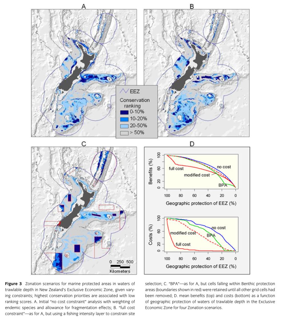
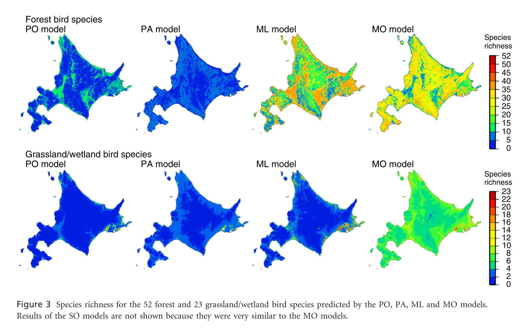
Declines in marine biodiversity due to human exploitation, especially in fisheries, pose a serious threat to our oceans. Marine Protected Areas (MPAs) are instituted in some areas in order to reverse these losses. Various methods are used to identify and justify new candidates for MPA status. This paper serves as a proof of concept, using the oceanic waters of New Zealand’s Exclusive Economic Zone, for a new method based on Species Distribution Modeling. Patchy locality data on 96 commonly caught fish species were interpolated across the EEZ using a Boosted Regression Trees based SDM based on environmental covariates functionally relevant to fish.  17,000 trawls were used for model fitting and 4,314 were used for model evaluation. Because of the zero inflated nature of the data two BRT models (the first was fit to presence absence in the trawl and the second to log of catch size given presence). After evaluation these models were used to make environment-based predictions of catch per unit effort for each species for 1.59 million 1km² grid cells. These predictions were employed for delineation of MPAs using the software Zonation. The software begins with preservation of the entire grid and then progressively removes cells that cause the smallest marginal loss to conservation value. The implementation used here attempts to retain high-quality core areas for all species. Of 96 predicted fish distributions 19 endemics were given higher priority weighting. Neighborhood losses were also assessed based on fish life histories such that the loss of some proportion of neighboring cells devalued the focal cell. The final component of the Zonation analysis is cost of preservation. The authors analyze outcomes under 4 cost scenarios: (1) “No cost restraint” equal costs for all cells so analysis is solely driven by species, (2) “full cost constraint” costs for grid cells varied based on fishing intensity, (3) “modified cost constraint” in which the costs of grid cells are rescaled from the “full cost constraint”, (4) “BPA” in which Zonation was used to assess the cost and value of a recently implemented set of Benthic Protection Areas in the waters around New Zealand.

Depth, temperature, and salinity contributed most to the predictive models. Models showed excellent predictive ability for presence/absence (Mean AUC=0.95, range= 0.86-0.99) but predictive ability for catch size was more variable (mean correlation= 0.534, range=0.05-0.82). “No cost constraint” analysis show that preservation of 10% of offshore parts of the EEZ would protect on average 27.4% of the geographic range of each of the analyzed fish species (46.4% if 20% is preserved). Use of neighborhood constraints identifies far more clumped groups of cells for protection. “Full cost constraint” analysis only shared 2/3 of its top 10% cells with the no constraint model but it would only provide slightly lower conservation value (mean=23.4% of each species range protected) with no loss of current fishing activity. “Modified cost constraint” analyses produced a range of intermediates between these two extremes. BPA areas (which comprise 16.6% of the trawlable EEZ) would protect on average 13.4% of species ranges if no fishing was allowed. Clearly all other scenarios outperform the current implementation of the BPA.

Maldonado, C., et al. (2015). “Estimating species diversity and distribution in the era of Big Data: to what extent can we trust public databases?” Global Ecology and Biogeography 24(8): 973-984.

The vast records of species distributions contained in natural history collections are rapidly getting digitized and becoming widely available online. These data provide an invaluable resource for Species Distribution Modeling. One of the largest biodiversity databases is the Global Biodiversity Information Facility (GBIF). Despite increasing quality of data researchers should retain a critical eye for poor quality of geographic positions or erroneous taxonomic identifications. The researchers ask to what extent data in the GBIF are sufficient for prediction of distribution patterns using data for the plant tribe Cinchoneae in the Neotropics. Three data sets were taken from GBIF: (1) a non-cleaned dataset (3720 records), (2) a cleaned dataset (3572 records), (3) and a cleaned dataset with the manual addition of records from other sources (3756 records). A fourth dataset (VD) was compiled manually through classical taxonomic work using the main herbaria in South America and the Missouri Botanical Garden (2670 records). Species distribution and species richness were analyzed on all four datasets at three spatial scales using SpeciesGeoCoder. Scales are grids (one-degree cells covering the entire range of the tribe), Ecoregions (defined by WWF), Biomes (polygons also defined by WWF). Distribution and richness were also analyzed by altitude. At the grid scale the basic GBIF data identified a number of richness hotspots not identified by VD these were noted to be a result of records with country level locality data which was converted to point data using the center of the country. These erroneous hotspots were not present after data cleaning because these rough locality measures were those preferentially cleaned. At the ecoregion level, in general, ecoregions in the central areas of a number of countries had higher richness under GBIF records than VD records as a result of the poor georeferencing described above. The number of species per ecoregion was not, however, consistently higher for GBIF. At the biome level the main discrepancy is a much larger number of species in the “Tropical and Subtropical Grasslands and Savannas and Shrublands” biome under VD (34) records than GBIF (10), again a result of georeferencing errors. As above the GBIF cleaned and GBIF cleaned and increased data sets more closely approximated VD. Increasing spatial scale did not ameliorate the effect of these errors. In contrast GBIF and VD widely concur in the altitudinal ranges of species.

GBIF records have the advantage of more participating institutions and consequently more records cheaply and in a uniform format but are still plagued by taxonomic and, most notably for this analysis, georeferencing errors. Data cleaning seems to deal with some forms of georeferencing errors relatively effectively. The authors also suggest raising minimum requirements for data submission and peer-review of data in order to increase GBIF data quality before the end user.

Acevedo, P., et al. (2012). “Delimiting the geographical background in species distribution modelling.” Journal of Biogeography 39(8): 1383-1390.

The role of the geographical background (GB) extent is clearly an important one in the field of Species Distribution Models. Notably an increased extent of GB can artificially inflate the perceived discriminatory power of an SDM by adding many uninhabited and unsuitable sites. And if unoccupied but environmentally suitable areas are used for model training then predictive capacity may be reduced. As an alternative to the methods of Barve et al. (2011) the authors propose trend surface analysis (TSA) as a way to determine the GB that maximizes the likelihood that the targeted species is interacting with the environment (i.e. areas that are otherwise accessible). The trial analysis was performed on four native ungulate species in mainland Spain. A third degree TSA was fitted (for processes that occur at the same or a higher spatial scale than the study area) the basic GB (GB_LOW) was delimited by selecting all points with the lowest TSA value assigned to a presence or greater. Then the GB was restricted by excluding 1%, 5% and 10% of the presences with the lowest TSA values and extended by including 1%, 5%, and 10% of the absences with the highest TSA values, lower than the value of any presence. Logistic regression models were trained on a 70% random sample fo the data. Predictive performance was assessed on three evaluation data sets: (1) the remaining 30% of the training data within the GB, (2) only evalutation data in GB_-10%, (3) using all the localities in GB_-10% for all species. TSA results showed broad-scale spatial trends in species distributions. Predictions of all models are quite similar in the core area and highest variability between different models is found when making predictions outside the training data sets. There was a negative association between AUC and GB extent when assessed on core areas and a positive association when evaluated on the training area. There was also a negative association between GB extent and the area of Spain predicted as suitable. Increasing GB produces models that appear better (higher AUC) but that are barely informative. Larger areas of suitability predicted by smaller GBs were also more in accordance with expert opinions. This TSA approach seems to offer a more easily implemented alternative to Barve et al. (2011) for estimating the parts of the landscape to be designated as ‘M’ or the accessible area and could perhaps be used effectively in a broad array of contexts.

Lennon, J. J., et al. (2011). “Are richness patterns of common and rare species equally well explained by environmental variables?” Ecography 34(4): 529-539.

Species richness predictions based on environmental models rely on the assumption that richness patterns of both common and rare species respond similarly to environmental variables. Additionally the contribution of rare species to variation in richness may be swamped out by the contributions of more common species meaning that environmental factors identified as important for richness may just be important for this small subset of influential species. This phenomenon may be driven by the skewed distribution of species commonness, namely that rare species are rarer than common species are common. So in a small assemblage of rare species there will be many areas with 0 richness, while a similar size assemblage of common species will have fewer areas of uniform richness (fewer 0s but still not many maximums). This paper focuses on showing how species along the rare-common continuum differ in environmental associations using grassland plant and lichen species along an environmental gradient on the Scottish island of South Uist. Hypothesis: Rare species associated with rare environments and common species with common environments and rare and common species differ in relation to environmental variable. 217 roughly evenly spaced samples were taken along a 200mX2162m grid. At each site species composition along with soil and environmental variables were recorded. To determine the effect of rarity on contribution to richness sub-assemblages were built sequentially from most common and least common species, correlated richness values for each individual sub-assemblage with the total assemblage and plotted them against rank order of species addition. In order to account for the relative capacity of species to contribute on the basis of their prevalence alone correlations were also plotted against the expected variance of the given sub-assemblage richness pattern. These correlation plots were compared to an iterated null model. Common species contribute more to species richness patterns than rare species. When expected variance due to prevalence is taken into account this pattern reverses for vascular plants with rare species more associated with higher richnesses. The rescaling of non-vascular plants that there may not be a clear relationship between rarity and richness. GLMMs with Poisson errors and exponentially spatially structured random affects fitted using penalized quasi-likelihood were fit to each pattern of building species assemblages, with species richness as response. Small assemblages of rare species are poorly explained by environmental covariates as compared to common species. For vascular plants richness vs. environment associations of common species differ from those for rare species. For non-vascular plants models fit to more common species fit better likely due to them being easier to predict. Similar GLMMs were fit to the relationship between the species richness of each assemblage along the rare-common axis as a function of the environmental rarity and extremity of the sample (in environmental space). For vascular plants, rarer species were significantly positively associated with extreme and rare environments while commoner species were associated with only moderate environments. For non-vascular plants, only common species were associated with moderate and rare conditions. This is despite the fact that environmental rarity and extremity are strongly correlated (r=0.84). Clearly common and rare species can both respond differently to environmental variables and differentially affect species richness while the responses differ between vascular and non-vascular plants.

Warton, D. I., et al. (2013). “Model-based control of observer bias for the analysis of presence-only data in ecology.” PLoS One 8(11): e79168.

Observer bias can be a major problem in building SDMs with presence-only data. The authors define observer bias as the idea that “a species is more likely to have been recorded as occurring in a place where people are more likely to see and record it.” Using presences for other sampled species as pseudo-absences for your model is one way of addressing this issue if we assume that observer bias is consistent across species. The paper considers two alternative ways of implementing this approach: a point based approach and a grid cell based approach (in which records within a grid cell are aggregated such that a presence point in a grid cell means that that cell is a presence record for the focal species or the non-focal species respectively). This approach may replace observer bias with species richness bias, by restructuring our question to one of species composition. We now ask, given we at least one species is present in a cell/point, what is the probability that it is our focal species. The authors, therefore, propose an alternative, model-based bias correction method which they compare with these earlier methods. This method consists of modeling the likelihood of observing a presence as a function of both environmental variables and “observer bias variables” such as accessibility of sites. These functions are assumed to be additive. In order to control for observer bias during prediction all observer bias variables are set to a constant across all prediction points/cells. All analyses are performed using a Poisson point process regression model with a LASSO penalty for variable selection. First the authors work through an illustrative example with a single species Eucalyptus apiculata. The model fit with environmental variables and the model fit with environmental and observer bias variables are relatively similar with the second providing a better fit to presence points. The model fit to both types of variables and then controlled for observer bias provides a very different distribution with positive predictions extending into low accessibility areas. In order to draw broader conclusions they trained and evaluated models using 5-fold cross-validation on a presence-absence data set containing 62 species. 84% of species were better predicted when using model-based bias correction than when ignoring bias. These improvements were on average relatively small (95% CI for increase in AUC: 1.5+/- 1.1). Significantly more species were predicted better by model-based bias correction than by the alternative pseudoabsence approach described above. Some species were, however, fit better by the pseudoabsence approach. Potential pitfalls of this new model-based bias correction approach include: a reliance on the quality of the variables chosen to quantify observer bias and on the ability for the effect of these variables to be estimated from the available presence records (making small numbers of records particularly problematic), and the reduction in effectiveness that will come from (likely quite common) correlations between environmental and observer bias variables. This method seems relatively effective and very well grounded conceptually. It would be interesting to see it compared to other common methods of bias reduction beyond the pseudoabsence approach.

The authors set out to test the performance of five presence-only and presence-background SDM methods on sparsely recorded species in the neotropics. They use presence data on the common anuran Hypsiboas bischoffi to test the building of SDMs for species in the Brazilian Atlantic Forest (BAF). The models that they compare include: BIOCLIM (envelope based method in environmental space), DOMAIN (distance based method in environmental space), SVM (non-probabilistic statistical pattern recognition algorithms for estimating the boundary of a set), OM-GARP (a genetic algorithm which selects a set of rules that best predicts the distribution), and MAXENT. In addition to simply comparing the performance of these models in this region they also compare two alternative “calibration” domains for their models, the BAF and all of South America. “Calibration” domains defined the region from which pseudoabsence points were chosen for evaluation as well for training of presence-background models (OM-GARP and MAXENT). For those models that use pseudoabsence (OM-GARP and MAXENT) they examine how increasing calibration area (background) changes predictions in environmental space. These questions are relevant particularly in the Neotropics and more broadly because of the importance of modeling relatively unknown species with distributions of unidentified extents. Evaluation was performed using 5 random 75% training -25% testing partitions with 10 random pseudoabsences per occurrence point and assessed via AUC. Mean AUCs of models ranged from .77 (BIOCLIM/BAF) to .99 (MAXENT/SA). AUCs were always higher for models calibrated in SA than those in BAF. SVM had the highest AUC for BAF (.95) while MAXENT had the highest for SA (.99). BIOCLIM had the lowest AUC for both domains. The highest difference in predicted area for BAF vs. SA was OM-GARP’s. MAXENT was substantially more robust in its environmental predictions than OM-GARP to changes in extent of background area. As a result both SVM and MAXENT seem to be good choices for SDMs regardless of the unknown extent of the true distribution while OM-GARP may be a good option when the “calibration” area concurs relatively well with the extent of the “true” distribution. The most interesting results of this paper are the differences between OM-GARP and MAXENT in the way that their predictions are affected by a change in the extent of background points. This serves as yet another strong argument for MAXENT as a great choice model. Most of the remainder of the results seem to distill to the fact that evaluating in an increased area ought to lead to higher AUC because there are more obvious absence areas that are easily identified.

Raes, N. and H. ter Steege (2007). “A null-model for significance testing of presence-only species distribution models.” Ecography 30(5): 727-736.

Validation of SDMs is both important and potentially difficult and problematic, especially in the case of presence-only data. Using pseudo-absence (background) points to calculate the AUC of trained models can create a number of problems, particularly that the maximum AUC is no longer 1 but rather 1-a/2 where a is the fraction of the landscape of interest genuinely covered by the species’ true distribution. As a result the interpretation of AUC values becomes muddied and typically “good” AUC values may not be what they seem. The authors propose a null model based approach to significance testing using “collection” localities, randomly drawn from the background, in equal number to the actual number of collection localities. This method relies, however, on the often unmet assumption that researchers have sampled all localities equally well. They propose to address this issue by drawing the random “collection” localities exclusively from the set of known collection localities. The authors illustrate this method using occurrences of the genus Shorea on the island Borneo and the SDM MaxEnt. They build both background based random null-models and null-models based on 1837 known collection localities for all plants across Borneo. Both of these types of null-models were used to construct a 95% confidence interval for AUC values such that AUCs outside of the interval implied that the model performed significantly differently from the random null model. 91% of species had a higher AUC than the random null-model CI, while only 61% had an AUC higher than the bias adjusted CI.  In so doing, they show the importance of correcting for bias in your presence points when building null models, while recognizing that often researchers will not have an accessible set of nearly 2000 potential collection points to use for correcting their null-model. They suggest using distance to features such as roads, rivers, cities, and nature reserves, as a proxy for this data. They found that the AUCs of their true models and both null-models decreased with increasing number of presence points (and growing predicted range size) which they interpret to mean that as the unknown true distribution of the species increases only the maximum AUC decreases and not the actual predictive ability of models. Though the concept of null-model based hypothesis testing has been used previously in SDM and elsewhere of course as well, the addition of the bias-corrected null model seems valuable for effective evaluation. It does ignore, however, the fact that the actual predictive accuracy of a given model will be affected by bias in the presence data. This method, though, may make our AUC evaluations more fair and accurate and so seems worth further study.

Fourcade, Y., et al. (2014). “Mapping species distributions with MAXENT using a geographically biased sample of presence data: a performance assessment of methods for correcting sampling bias.” PLoS One 9(5): e97122.

http://journals.plos.org/plosone/article?id=10.1371/journal.pone.0097122

Fourcade et al. attempt to assess the effectiveness of a number of methods for correcting sampling bias in species distribution modeling with MaxEnt. Bias in species sampling has been well established as an important and difficult problem in species distribution modeling. The authors take large, and likely spatially unbiased, presence only sample sets for 1 virtual and 2 real species and impose 4 types of spatial bias on them to simulate sampling bias. These types of biases are (1) Two Areas, the northern region has high sample density and the southern region low density, (2) Gradient, a density gradient decreasing from north to south, (3) Center, the density decreases gradually from the core of the distribution to the edges, (4) Travel Time, probability of keeping a record was highest when it had the lowest travel time to the nearest city. 5 different data-processing methods were used to limit the effect of these spatial biases: (a) Systematic Sampling, a grid of a defined cell size was superimposed on the distribution and 1 record was chosen per grid cell, (b) Bias File, MaxEnt can be given a file representing sampling effort with which it weights the sampled points, (c) Restricted Background, MaxEnt’s background points were drawn exclusively from buffer areas around biased occurrences, (d) Cluster, a PCA was performed on the environmental predictors then occurrence points were analyzed for clustering in the 2 dimensional environmental PCA space and 1 record was randomly sampled per cluster, (e) Split, occurrences were split into a northern and southern group and MaxEnt was applied independently to each area. These methods all seem relatively well grounded individually but the combination fails to make much sense. Most notably, it is entirely unclear why grid based selection is used for spatial thinning and cluster analysis for environmental thinning. Models were compared using AUC, overlap species probabilities in environmental (Denv) and geographic (Dgeo) space. Biased models invariably had lower AUCs than unbiased models and clearly deviated from the unbiased model by all measures. Decrease in AUC, however, was small and the AUC of biased models was usually still in the range generally accepted as a well fit model. The effect size of each bias type depended on the species and evaluation method. The authors focused on Dgeo (Denv was strongly correlated) as the main measure of effectiveness of bias correction. Overall only 29% of all combinations (species*bias type*bias intensity*correction method) showed improvement over the biased model with the simulated species substantially easier to correct (57% were successful corrections). Restricted Background (c) failed in almost all cases (6% successful). All other methods performed better but were differentially ranked depending on the combination of factors. Systematic sampling (a), though not always ranked first, performed most consistently and slightly better overall than the competing methods (33% successful). Bias file (b) and cluster (d) methods sometimes outperformed Systematic Sampling but were slightly less successful overall (23%, 23%). Probably the most important result of this work is the bad performance of the Restricted Background (c) method, as it seems to be consistently used/recommended when fitting MaxEnt to biased data. Though Systemtatic Sampling (a) performs well and consistently, the authors acknowledge that the second main conclusion is that the best way of handling bias is often context specific and so one ought to attempt multiple different correction methods in practice. Their somewhat strangely chosen set of correction methods further reinforces this point as other methods that have been demonstrated as effective went untested or were replaced with minor variants that may have changed their effect.

Wisz, M.S., Hijmans, R.J., Li, J., Peterson, A.T., Graham, C.H. and Guisan, A., 2008. Effects of sample size on the performance of species distribution models. Diversity and Distributions, 14(5), pp.763-773.

http://onlinelibrary.wiley.com/doi/10.1111/j.1472-4642.2008.00482.x/pdf

Wisz et al. set out to address the ways in which limited sample size (which is often a problem when constructing Species Distribution Models) on model performance. The importance of sample size to SDM comes in the fact of the lower uncertainty of parameter estimation with increasing sample size. This importance is compounded by the high dimensionality of the environmental space often being modeled and the fact that the interactions between multiple environmental dimensions are often important. All this serves to increase the total number of parameters to be estimated, placing further demands on sample size. Therefore, the authors chose to test the sensitivity of 12 different species distribution models (see Table 1 in paper for full list) to sample size variation. Models were trained with presence-only data from natural history collections and evaluated with independent presence-absence data from planned surveys, via AUC. All 12 models were trained on 10, 30, and 100 randomly sampled presence points for each species. Each of these training subsets was evaluated for its degree of overlap in environmental space with the evaluation points for that species. Finally, linear mixed effects models were used to determine which factors significantly affect AUC. Smaller sample sizes exhibited significantly lower environmental range overlap than larger samples. LMEs showed a significant effect of the interaction between modeling method and sample size. Nearly all algorithms performed better with more records (exceptions being DOMAIN and LIVES). MaxEnt performed best at low sample sizes and was the second best performer at intermediate and high sample sizes (outperformed by GBM) with intermediate variances at all sizes. BIOCLIM exhibited the lowest variance across all models but also very low AUCs. At 10 records MAXENT, OM-GARP, and DOMAIN all had high AUCs with intermediate variances. As expected, methods that model complex predictor relationships were particularly sensitive to sample size (e.g. GAM, GBM, BRUTO). A major open-ended question of the work is what the difference between randomly subsetted data and “naturally data-depauperate” species records resulting from biological rarity. It stands to reason that the above analyses may not accurately apply to such a situation.