What do we gain from simplicity versus complexity in species distribution models?

Merow, Cory, et al. “What do we gain from simplicity versus complexity in species distribution models?.” Ecography 37.12 (2014): 1267-1281.

A variety of methods can be used to generate Species distribution models (SDMs), such as generalized linear/regression models, tree-based models, maximum entropy, etc. Building models with an appropriate level of complexity is critical for robust inference. An “under-fit” model will introduce risk of misunderstanding factors that shape species distribution, whereas an “over-fit” model brings risks inadvertently ascribing pattern to noise or building opaque models. However, it is usually difficult to compare models from different SDM modeling approaches. Focusing on static, correlative SDMs, Merow et. al. defined the complexity for SDM as the shape of the inferred occurence-environemnt relationships and the number of parameters used to describe them. By making a variety of recommendations or choosing levels of complexity under different circumstances, they developed negeral guidelines for deciding on an appropriate level of complexity.

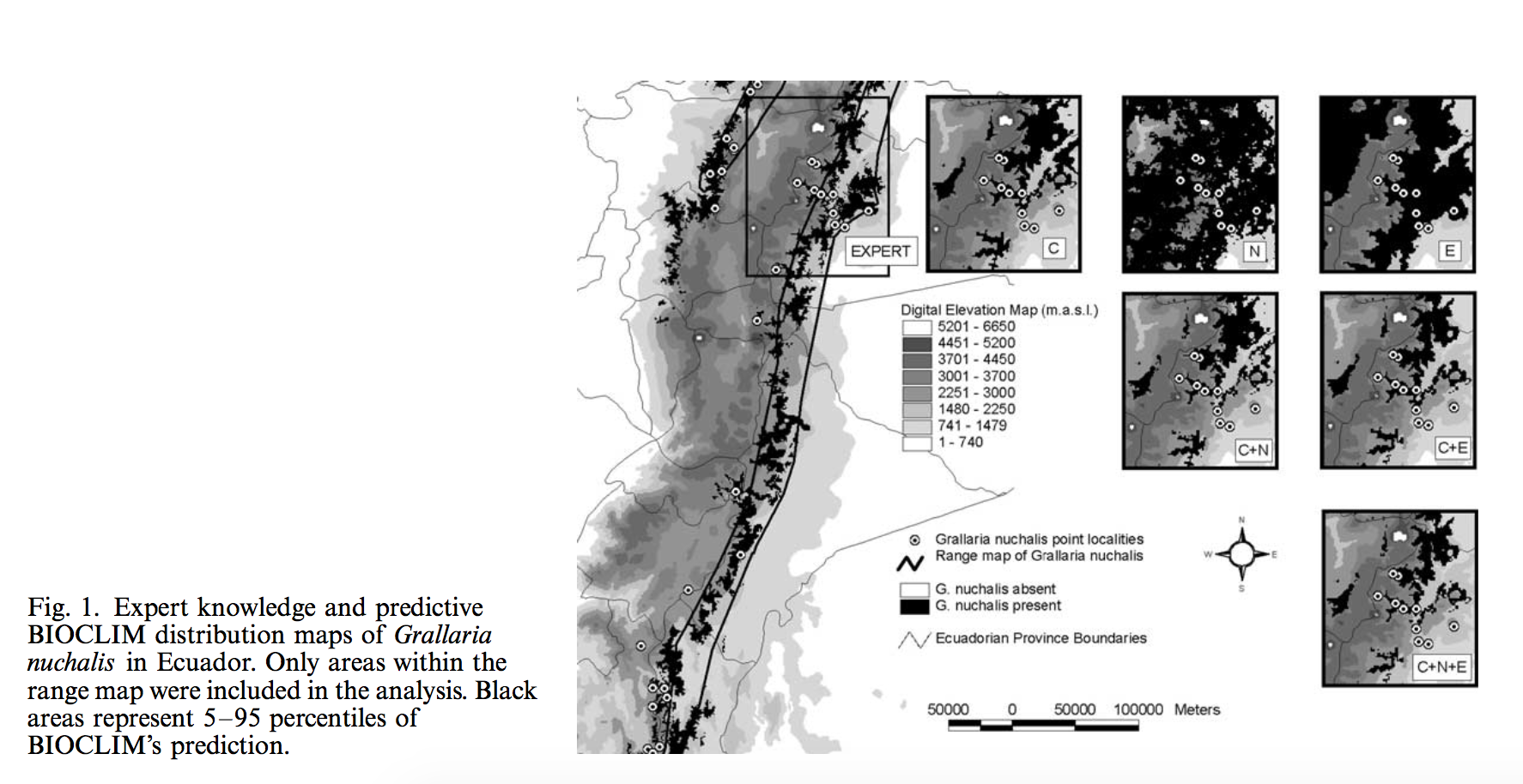
There are two attributions determining the complexity of inferred occurrence-environment relationships in SDMs: the underlying statistical method (from simple to complex: BIOCLIM, GLM, GAM, and decision trees) and modeling decisions made about input and settings. As for modeling decision, larger numbers of predictors are often used in machine-learning methods instead of traditional GLM. Incorporating model ensembles and predictor interactions will also increase model complexity.


Screen Shot 2016-02-10 at 1.39.59 PM

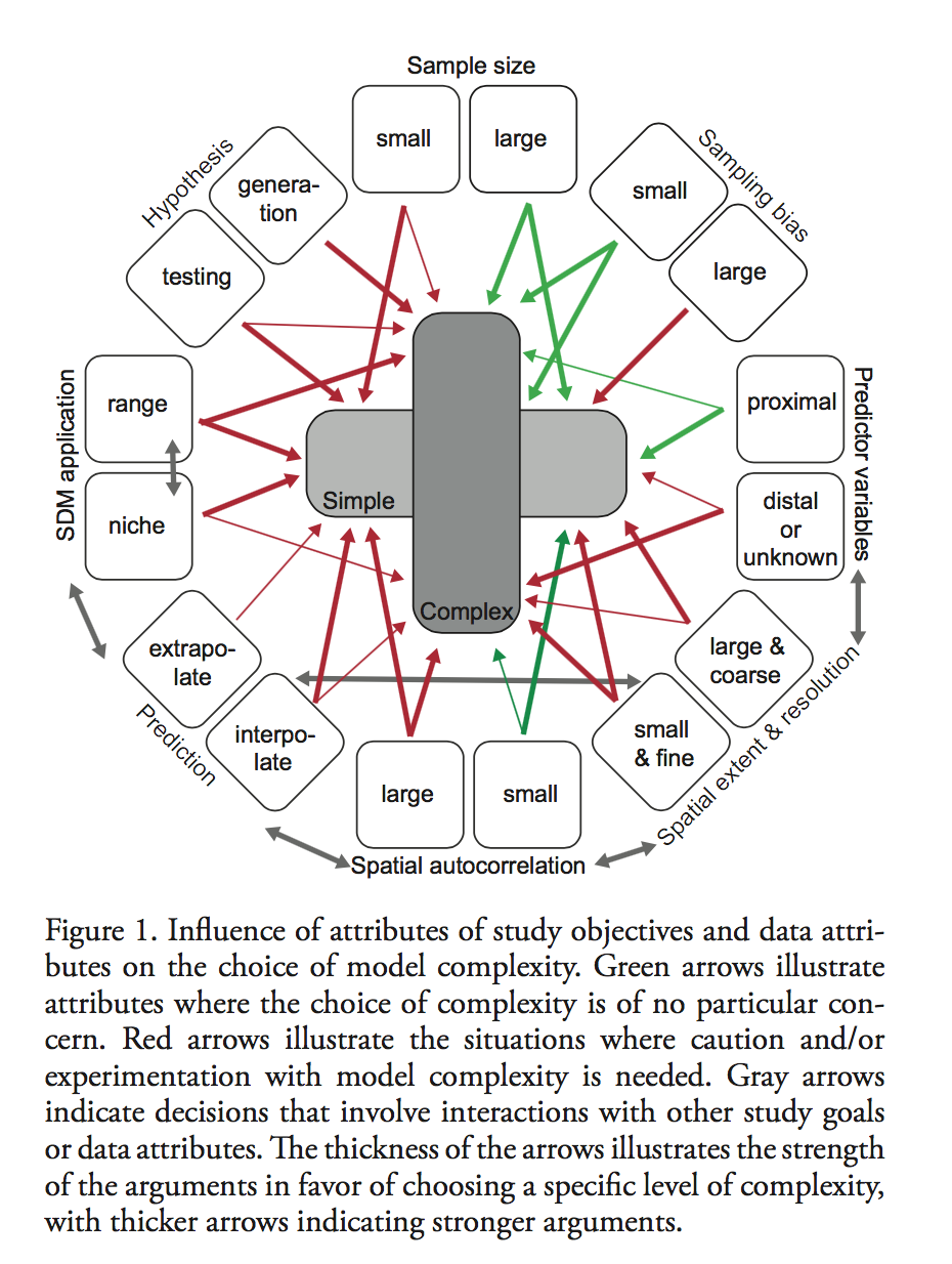
Figure 1 summarized their finding in terms of general considerations and philosophical differences underlying modeling strategies. They suggested that before making any decisions on model approaches, researchers should experience both simple and complex modeling strategies, and carefully measure their study objectives (Niche description or range mapping? Hypothesis testing or generation? Interpolate or extrapolate? ) and data attributes ( sample size, sampling bias, proximal predictors and distal ones, spatial resolution and scale, and spatial autocorrelation). Generally speaking, complex models work better when objective is to predict, and simpler models are valuable when analyses imply only certain variables are needed for sufficient accuracy. Finally, they concluded that combining insights from both simple and complex SDM approaches will advance our knowledge of current and future species ranges.

Relating this paper with the Breiman paper, Merow et. al. regarded data modeling models simpler than algorithmic models, which are usually semi- or fully non-parametric. But they also acknowledged that this conception is rather relative: the interpretability of complex models is not necessarily difficult, and the complexity can still identify simple relationships. However, it can be seen that Merow et. al. regarded interpretation of models one of the goals of modeling. They think there is no absolute situations that simple models or complex models violate the nature of science, but their merits are more case-dependent. I think the combing of simple and complex models, as Merow et al suggested, is the trend of statically modeling, and Breiman maybe over-emphasized the distinctions between the two cultures in modeling world.

Not as good as they seem: the importance of concepts in species distribution modeling

By comparing existent models, some ecologists found that complicated modeling techniques are more robust in terms of realized distribution modeling, and that predictions are usually more reliable for the species with smaller range sizes and higher habitat specifity. Jimenez-Valverde, Lobo, and Hortal argued that the interpretation of modeling results found in the comparisons above would vary if methodological and theoretical considerations are taken into consideration. They mentioned three important topics that need to be taken into consideration when conducting species distribution modeling: 1) the distribution between potential and realized distribution, 2) the effect of the relative occurrence area of the species on the results of the model performance, and 3) the inaccuracy of the resulted prediction of the realized distribution from different modeling methods. They reviewed most recent papers applying SDMs and discuess the negative implications of neglecting the three issues mentioned above, targeting on two general conclusions from other comparison papers:

– Are complex techniques better for the prediction of species distributions than simple ones?

With the bias shown by most of the biodiversity inventories, any comparisons among presence-only modeling generally provide distribution close to the potential. A more complex technique tends to overfit the presence data. When validate it with true absence data, it can be erroneously concluded that the predictions from the complex one are more accurate.

– Are the predictions fro specialist species more reliable than for generalists?

Jimenez-Valverde et.al. argued that the seemingly better predictions for specialists are usually the result of the properties of the data used for validation. Besides, rare/specialists and common/generalists gradients are extent- and scale- dependent. They found models of rare species are inevitably with high discrimination, which would be either over or underestimate the distribution of the species.

Their conclusion is that a solid conceptual and methodological framework is necessary for future works evaluating, comparing, and applying species distribution modeling techniques. This paper is inspiring since it provided alternative explanations for universally admitted conclusions. It will be more convincing that they can have species example as supports for their theoretical arguments. In addition, they “deliberately avoided using the term niche to refer to species distributions” due to the recognition that species can be absent from suitable habitat and/or present in unsuitable ones. So they clarified that they were only talking about statistical models, which are not able to provide a description if species niche. It is kind of ironic that they supported a “better understanding of basic concepts for any species modeling or methods comparison” on one hand, and avoided to talk about the most basic concepts behind distribution theory on the other hand.

Modelling species distributions without using species distributions: the cane toad in Australia under current and future climates

Almost all approach for GIS-based distribution modeling depend in some way on species occurrence data. In range-shifting species, however, the correlative approach usually requires extrapolation to novel environments, which could lead to erroneous predictions. Kearney et. al. used an alternative approach with emphasis on the ecology of organisms based on ecophysiology and organism traits, which is independent from species current distribution. They used fine-resolution spatial dataset together with a set of biophysical and behavioral models to make the predictions of Cane Toads distribution under current and future climate in Austrilia, assessing the direct climatic constraints on their ability to move, survive, and reproduce. The results show that the current species range can be explained by thermal constrains for the adult stage and water availability for the larval stage. Their research provided a framework showing trait-based approaches can be used in investigates the range limits of any species by quantifying spatial variation in physiological constraints and therefore defining regions where survival is impossible. They claimed that mechanistic approaches have broad application to process-based ecological and evolutionary models of range-shift. In my opinion, an effective mechanistic model depends on sophisticated observational or empirical data to from the mechanism of the target organism, which maybe not that easy to obtain for all kinds of species. In addition, researchers could never capture all factors for the fundamental niche. The way Kearney et. al. addressed this problem is by identifying areas outside the niche and to locate impossible areas for the organisms. Therefore, their predicted areas are less restricted than the actual range.


Screen Shot 2016-01-27 at 12.00.43 PM


Kearney, M., Phillips, B. L., Tracy, C. R., Christian, K. A., Betts, G., & Porter, W. P. (2008). Modelling species distributions without using species distributions: the cane toad in Australia under current and future climates.Ecography, 31(4), 423-434. DOI: 10.1111/j.0906-7590.2008.05457.x

Evaluating alternative data sets for ecological niche models of birds in the Andes

Typically, researchers use interpolated climate data or remotely sensed environmental data to build Ecological niche models (ENMs). Parra et. al. conducted the first assessment of the relative performance of models created by three different datasets: climate data, Normalized Difference Vegetation Index (NDVI), and elevation data. They compared predicted versus expected distribution of six bird species in the Ecuadorian Andes. They developed seven models based on three datasets and all their combinations using BIOCLIM. Predictive maps were compared with expert knowledge based maps, and sensitivity, specificity, positive predictive power, and Kappa were calculated. They found that models included climate variables performed well across most measures, whereas ones only use NDVI performed the worst. In the mean while, elevation data based models showed high over-prediction errors. They concluded that it is usually beneficial to include various datasets into ENMs when possible. Data quality of remote sensing data should be evaluated carefully before being included, especially for regions with complex topography or cloudy weather. This comparison result, however, may revealed a regional trend for Ecuadorian Andes but not a general rule, considering the special landscape, high levels of endemism, and species richness of the study area. Therefore, similar modeling comparison will benefit further understanding for effects of data choosing on ENMs.

Screen Shot 2016-01-19 at 10.26.49 PM

The role of land cover in bioclimatic models depends on spatial resolution

DOI: 10.1111/j.1466-8238.2006.00262.x

The spatial scale on which species distribution modeling is undertaken is of fundamental importance for ecological studies. The current paradigm indicates climate governs species distribution on broad biogeographical scales whereas land cover and habitat suitability affect species occupancy patterns, especially at fine resolution. With this context, Luoto et. al. tested whether the integration of land cover data affect bioclimatic models by constructing Generalized additive models for 80 bird species as a function of (1) pure climate and (2) climate and land cover variables. Models were constructed at 10km, 20km, 40km, and 80km resolutions. They evaluated their models using area under the curve (AUC), and found that model performance generally increased when land cover was included at 10km and 20km. In contrast, the inclusion of land cover decreased model AUC at 80km resolution. Therefore, they concluded that the determinants of bird species distributions are hierarchically structured, and that integrating land cover at 10km-20km resolution can improve our understanding of biogeographical patterns of birds in their study area. This paper examined effects of spatial resolution over a range of scales. However, whether a certain spatial resolution is fine or course is species-dependent and question-driven. It would be interesting to discuss about a protocol that help determine appropriate spatial scale for general species distribution modeling.

2 (1)
Projected distributions of two species with different modelling accuracies and habitat preferences: the occurrence of marsh harrier (Circus aeruginosus): (a) climate model and (b) climate-land cover model; and the occurrence of grey-headed woodpecker (Picus canus): (c) climate model and (d) climate-land cover model. Black dots represent the sampling plots where the species was present, and shaded areas are the areas modelled as suitable for the species. To determine the probability thresholds at which the predicted values for species occupancy are optimally classified as absence or presence values, we used prevalence of the species as the probability level as suggested by Liu et al. (2005). D2 = percentage of explained deviance and AUC = the area under the curve of a receiver operating characteristic (ROC) plot.