Selecting thresholds for the prediction of species occurrence with presence-only data

Liu, C., White, M., & Newell, G. (2013). Selecting thresholds for the prediction of species occurrence with presence-only data. Journal of Biogeography, 40(4), 778–789. http://doi.org/10.1111/jbi.12058


Many of the newer methods for SDM output continuous values, but binary predictions are often needed in application and when evaluating models, necessitating the need for thresholding. Many thresholding techniques have been proposed, such as lowest presence threshold, fixed thresholding, and minimizing or maximizing a the difference between opposing statistics, but there is no consensus on which performs better, and presence-only data can not be used in all of these instances. Liu et al (2013) compared 12 different techniques through mathematical proofs and simulations of species distributions. First, they use mathematical proofs to show that only eight of the techniques will result in similar thresholds using presence-only and presence-absence (or pseudo-absence) data. They then use 1000 simulated data sets of species occurrences to evaluate the variation within each thresholding technique, based on eight modeling approaches: Mahalanobis distance, ecological niche factor analysis, and GAM and random forest, the final two which each had three models using presence/absence, presence/pseudo-absence, and presence/psuedo-absence filtered with Mahalanobis distance. They choose four techniques (max kappa, min D01, meanPred, and max SSS) to evaluate. To sum up their (many) results, max SSS (which maximizes the sum of sensitivity and specificity) was most robust to pseudo-absences and changes in species prevalence, meaning it had less variation in its threshold definition as those parameters changed. When evaluated on the criteria of objectivity, equality, and discriminability, it performed better than the other methods because it is objective, unaffected by pseudo-absences, and produced higher sensitivity and specificity than other methods. All of the thresholding methods, however, are influenced by sampling bias in environmental space, especially as the sample size decreases. Based on all of the caveats to thresholding, I think it would be best to avoid doing unless absolutely necessary or to offer results based on multiple thresholds. When this is unavoidable, max SSS will perform the best.

Statistical solutions for error and bias in global citizen science datasets

Bird, T. J., Bates, A. E., Lefcheck, J. S., Hill, N. A., Thomson, R. J., Edgar, G. J., et al. (2014). Statistical solutions for error and bias in global citizen science datasets. Biological Conservation, 173(C), 144?154. http://doi.org/10.1016/j.biocon.2013.07.037


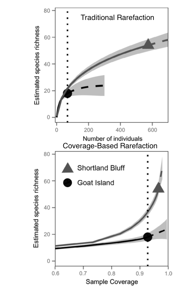
Citizen science has been gaining traction because of its ability to be both an outreach and data collection tool, however there is a serious concern about bias in the data. This bias can be avoided by implementing trainings and stricter sampling protocols, or through statistical processes more often used to correct sampling bias in SDM. The primary issues in citizen science data are greater variability and sampling bias. Fortunately, many of the same statistical methods for accounting for bias in normally gathered occurrence data can be used for citizen science data. We’ve discussed many of them in more detail in class, so I will only focus on the more novel techniques. One method they recommend is accounting for variation between surveyor’s skill levels or biases by using mixed-effects models where surveyor identification is a random effect. Because citizen science data is usually less sparse than normal occurrence data, another common technique is to use an occupancy-detection model, which is based on other citizen scientists’ data. Similarly, when calculating biodiversity or species richness, you can account for under sampling by using a measure of sample “completeness”, similar to conventional rarefaction curves, but which extrapolate species richness before limiting the samples, resulting in higher species richness measures (see Figure). While these statistical methods allow for some correction, they can not completely correct for bias in citizen science data as well as proper training of volunteers and protocols. AS citizen science becomes more well-used, a field of comparing citizen science data to expert data is growing, which will hopefully be able to inform and better design citizen science experiments to mitigate these issues from the beginning.

for blog

Do Ecological Niche Models Accurately Identify Climatic Determinants of Species Ranges?

Searcy, C. A., & Shaffer, H. B. (2016). Do Ecological Niche Models Accurately Identify Climatic Determinants of Species Ranges? The American Naturalist, 187(4), 1–13. http://doi.org/10.5061/dryad.667g2


A major question surrounding ecological niche modeling is if models accurately reflect the biological ranges of species and if they are informative regarding a species niche requirements. If they do reflect these ecological “truths”, and not simply correlations with climatic variables, then their use in the prediction of species ranges into future climatic conditions is valid. To explore this issue, Searcy & Shaffer (2016) compare climatic variables that determine recruitment in the field with those predicted as high ranking by MaxEnt. Using two decades of demographic data on the endangered California Tiger Salamander, the authors replicated BioClim variables using climate data from nearby weather stations and ran ANCOVA models to measure how well a climatic variable correlated with juvenile recruitment of the salamander. They then created two MaxEnt models:
– a basic model that used permutation importance to rank variable importance
– an informed model that used permutation importance and percent contribution to rank variable importance, and
– corrected for sampling bias
– limited background points based on natural history of the species
– used model selection to select the model’s regularization multiplier

They then compared the variable importance rankings from the ANCOVA models to the two MaxEnt models, evaluating ranking and the response curves, the latter to see if the relationship between the variable and habitat suitability/recruitment was the same.

They found six variables to be highly correlated with recruitment, and these six variables were highly correlated with those predicted as important by MaxEnt, when using the informed model with importance by permutation. Notably, this was not seem with the other models, suggesting that an informed model using permutation may best illustrate biological realism. Interestingly, the response curves were not all the same, with temperature variables exhibiting similar response curves, but precipitation variables correlated in opposite directions. This may be due to the fact that they only considered linear responses, effectively dropping most MaxEnt curves, which were non-linear. It may also be due to the temporal scale of rainfall, in which one year with above-average rainfall can lead to high population growth, but an overall increase in rainfall over many years can decrease population growth.

In general, this paper provides evidence that ENM is based on biological realism, albeit with several caveats. Only the informed MaxEnt model with permutation reflecting this conclusion, suggesting that variable ranking by permutation should always be chosen, and models should be corrected for sampling bias and natural history, and controlled with a regularization multiplier. It also stresses that many biological responses are non-linear, so any models that treat them as such are likely to fail.

Note: They also use the MaxEnt model to predict the effect of climate change on the salamander, but this seemed less relevant and generalizable to the class, so I didn’t report on that aspect.

Socioeconomic legacy yields an invasion debt

Essl, F., Dullinger, S., Rabitsch, W., Hulme, P. E., Hulber, K., Jarosik, V., et al. (2011). Socioeconomic legacy yields an invasion debt. Proceedings of the National Academy of Sciences, 108(1), 203–207. http://doi.org/10.1073/pnas.1011728108


Human activities play a large role on the distribution of species, however, this relationship is often characterized by a time lag. One such relationship is the “extinction debt” in which a species is “committed” to extinction following fragmentation or disease, but is not yet extinct. A similar phenomenon may occur for an invasive species before it becomes established, described by the authors as an “invasion debt”. To test the hypothesis of the existence of an “invasion debt” due to anthropogenic activities, Essl et al. compared two spatially explicit models relating socioeconomic activity in current (2000) and historical (1900) time periods to current invasive species richness, with superior model performance by the historical model as evidence of an invasion debt. The study focused on invasive species of Europe, studying ten taxonomic groups, both individually and aggregated, in twenty-eight countries. In order to correct for correlation of socioeconomic variables, the authors created three PCA axes for the three variables, however, they still found the axes to be highly correlated over time (ie wealthy countries in 1900 were wealthy in 2000, which is to be expected). When considering an aggregation of all ten taxonomic groups of species richness as the response variable, Essl et al. used a linear mixed effects model, accounting for spatial autocorrelation with an “exponential within-group correlation structure”. This seems to be a correction to the response variable itself, which Beale et al. showed to reduce a model’s precision, however there is not enough detail in the methods for me to be sure. Spatial autoregressive models were fit for individual taxonomic groups using countries’ capitals as the spatial locations, correcting for correlation in the error term using a neighborhood matrix. The geographical location of a capital seems to be a very coarse measurement, yet it does match the national scale of the species richness data and capitals, being trade hubs, may be likely introduction points for many invasive species. The model of all ten groups combined found the historical model to have a lower AIC score. Combined with the fact that most species introductions occurred after 1950, this suggests the presence of an invasion debt. This seemed somewhat counterintuitive, however, I believe the authors view the invasion debt not as the time between an introduction and establishment, but as a “legacy effect” that may make an area more prone to invasion, perhaps through an increase in invasive pathways or habitat disturbance and fragmentation. Interestingly, when subdivided into taxonomic groups, reptiles and birds show the opposite relationship and are better predicted by the more recent socioeconomic PCA axes, which may be caused by the role of the pet trade, a more recent establishment, in their invasion success.

Food for Thought: This paper brings two things to mind with regards to 8910. First, that legacy effects may be an important aspect to consider when modeling the potential distribution of invasive species. For example, if historical economic activity is shown to be a predictor of current species distributions, more recent activity may increase accuracy of future distributions. Second, this study seems to incorporate spatial correlation in a way opposite to that recommended in Beale et al. 2010. This leads me to wonder if they are correcting for spatial correlation incorrectly, or if the principles used in SDM are not generally applicable to other types of spatial data.

MaxEnt versus MaxLike: empirical comparisons with ant species distributions

Fitzpatrick, M. C., Gotelli, N. J., & Ellison, A. M. (2013). MaxEnt versus MaxLike: empirical comparisons with ant species distributions. Ecosphere, 4(5), art55–15. http://doi.org/10.1890/ES13-00066.1


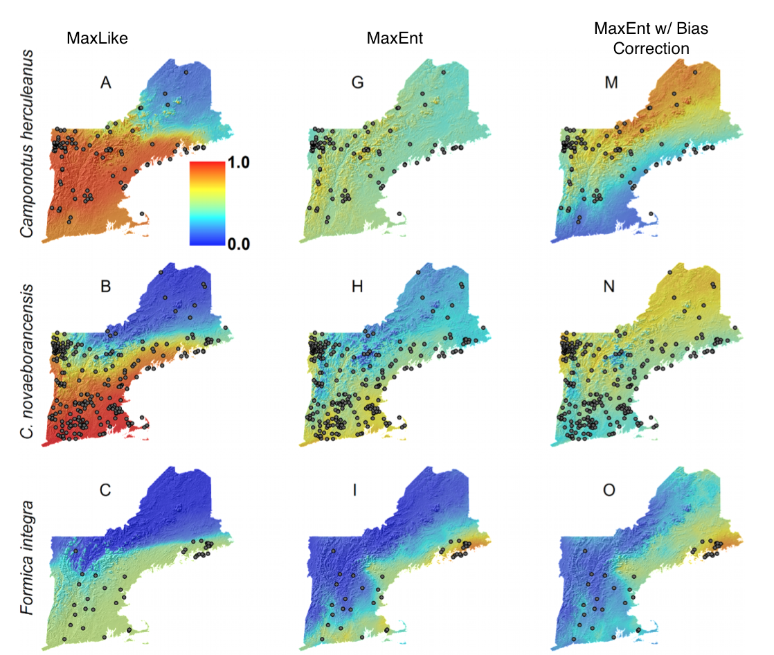
The output indices of MaxEnt are not truly direct estimators of the probability of species occurrence, but rather “ill-defined suitability [indices] (Royle et al 2012). In response to this, MaxLike, a formal likelihood model that generates ‘true’ occurrence probabilities using presence-only data, has been proposed as an alternative and shown to generate range maps that more closely match those of logistic regression models. However, it is unclear whether it can be generalized to SDMs to the extent that MaxEnt has been because the only comparison case so far used a larger sample size than is most often available, included the full geographic range of the species (and most studies cannot), and modified MaxEnt’s default settings, which may have reduced MaxEnt’s performance. As a test of generalization, Fitzpatrick et al compared MaxEnt andMaxLike models for six species of ants in New England, comparing outputs with goodness of fit, predictive accuracy measures, and comparison to expert opinion.

The authors began with 19 environmental variables, but then reduced to three: Annual Temperature and Rainfall, and Elevation. In doing so, they may have biased their study, as MaxEnt may be more robust to having multiple correlated or irrelevant variables than MaxLike. They then created 50 MaxEnt and 50 MaxLike models. The default settings were chosen for the MaxEnt models, and created a sampling bias surface based on the full dataset of ant occurrence records for 132 species was used to correct bias. Interestingly, a bias surface of all 132 species decreased MaxEnt performance, perhaps becuase the bias of the six focal species did not match that of the full dataset. Indeed, when the model was fit with a bias surface of only six species, it was a marginal improvement over the non-bias corrected models.

Goodness of fit was calculated with AIC and normalized Akaike model selection weights. Because AUC is especially problematic with presence-only data (WHY), two other measures of accuracy, minimum predicted area and mean predicted probability, were also examined. The authors have been working in this ant system for decades, so they were also able to compare models of distribution to expert knowledge and experience, a rarity, in my opinion, as many modelers are using data from systems they are unfamiliar with.

MaxLike models were better supported by the data, but model evaluation by AUC was inconclusive, although generally bias correction decreased the AUC of MaxEnt. In general, MaxEnt underestimated the probability of occurrence in areas where there were presence records, but over-estimated in unsampled areas. This is most likely due to the fact that MaxEnt assumes a mean probability of 0.5 for presence data, reducing the range of occurrence probabilities. Even with small data sets (to a minimum of five presence points) MaxLike more accurately predicted occurrence probabilities. Notably, because the authors created 50 models of each, a measure of uncertainty is available. In general, MaxLike had greater uncertainty, especially in areas with few presence points, which seems to be a fair and accurate conclusion to be drawn that machine learning methods often omit. MaxLike is able to perform better than MaxEnt on sparse data sets, even when MaxEnt is fit using default settings, and has the additional benefit of portraying uncertainty more accurately.

Comparison of occurence probabilities for MaxLike, Maxent, and Maxent corrected for sampling bias

The landscape configuration of zoonotic transmission of Ebola virus disease in West and Central Africa: interaction between population density and vegetation cover

Walsh, M. G., & Haseeb, M. A. (2015). The landscape configuration of zoonotic transmission of Ebola virus disease in West and Central Africa: interaction between population density and vegetation cover. PeerJ, 3(1), e735–13. http://doi.org/10.7717/peerj.735


Following the epidemic outbreaks of Ebola Virus Disease (EVD) in West Africa in 2014, it is obvious that the ability to predict, and perhaps even prevent, such outbreaks could greatly inform public health efforts, and save lives. Walsh & Haseeb (2015) use a point process distribution model to understand what are the socio-ecological drivers of zoonotic transmission events of EVD. Unique transmission events were recorded from the PubMed Database and World Health Organization reports, and matched to a geographical location. The authors chose three types of covariate data: WorldClim data on temperature and precipitation, Maximum Green Vegetation Fraction from Modis as a measure of vegetation, or forest, cover, and population density data from the Global Urban-Rural Mapping Project. First, they created a homogenous Poisson process (ppm), which served as a null model because the expected number of location points scaled with the area of the subregion, and inhomogenous Poisson process, which incorporate spatial dependence into the location of transmission events. The inhomogenous ppm fit the data better, and then was then expanded to include the four covariates listed above, plus altitude and an interaction covariate between vegetation cover and population density. The ppm allowed for the use of conventional statistical tests of significance, such as p-values and confidence intervals. Three covariates came out as important. Both increasing population density and increasing vegetation, although slightly less so, cover corresponded to a decrease in spillover risk. Interestingly, the interaction between these two variables was also significant, implying that the ‘protective effect’ of vegetation cover decreases with increasing population density. This suggests the presence of ecotones, where denser human populations are coming into contact with recently fragmented forest, an avenue for zoonotic spillover that has been suggested in the past.

Thoughts: An ecological niche model of EVD has been described previously, but this study incorporates the additional complexity of social factors, which I believe is especially important when considering spillover events. Doing so, however, removes distribution modeling from this idea of a fundamental niche, in my opinion, because it is no longer simply where EVD can persist but where it spills over. Semantically, this could be a ‘niche’ for spillover events. I also think it is important that they considered interactions amongst environmental covariates, especially because certain variables are correlated or depend on others.

The study’s code is online with data, if anyone is interested in reproducing it or just playing around point process models.

Forecasting Chikungunya spread in the Americas via data-driven empirical approaches

Escobar, L. E., Qiao, H., & Peterson, A. T. (2016). Forecasting Chikungunya spread in the Americas via data-driven empirical approaches. Parasites & Vectors, 1–12. http://doi.org/10.1186/s13071-016-1403-y


The goal of this paper was to predict the spread of Chikungunya in the Americas during the epidemic using 1) ecological niche models of Aedes aegypti and Aedes albopictus, 2) air travel data as a measure of imported cases and 3) fitted curves to reported CHIKV data as a measure of local transmission.  Case data was reported from the Pan-American Health Organization by country for the Americas.  In addition to the lack of standardization in reporting, the case data showed ‘surveillance fatigue’, in which reporting became erratic and uneven in the later stages of the epidemic, suggesting that reports from earlier in the epidemic may create more accurate models. By combining imported and local cases, the model predictions based on earlier reports matched later case data, suggesting that air travel is an important and accurate predictor of country-to-country transmission.

The ecological niches were estimated using climate envelopes, which create ellipsoids, similar to a convex hull method.  The minimum-volume ellipsoid method of climate envelopes creates semi-axes which reduce the Euclidian distances between occurrence points in environmental space. Rather than using all of the WorldClim variables, the authors used a principle components analysis to reduce any correlation amongst them, and chose the first three principle components as their environmental axes. The authors chose to use occurrence data from the global distribution of the vectors, in an attempt to estimate the fundamental niche and not the realized niche.  The output of the climate envelope was a niche centroid, where the semi-axes crossed in environmental space.  Hotspots were defined as areas closest to the niche centroid in environmental space.  It seems, then, that the envelope is not a boundary classifier, but ranks locations based on distance to the niche centroid, so may not perform as well at the edges of the species range as estimators such as support vector machines. They found that the niche models generally agreed with CHIKV case data, with areas closest to the niche centroid in the Carribean, where CHIKV was first introduced in the Americas.

The use of a minimum-volume ellipsoid was well suited to the study of the start of the CHIKV epidemic because this is also the area most well-suited for the vector.  I do not think it would be as appropriate when applied to more temperate areas further from the niche centroid, because the centroid seems to be where the model is most accurate.

Ecological niche and potential distribution of Anopheles arabiensis in Africa in 2050

Drake, J. M., & Beier, J. C. (2014). Ecological niche and potential distribution of Anopheles arabiensis in Africa in 2050. Malaria Journal, 13(1), 213–23. http://doi.org/10.1186/1475-2875-13-213


Anopheles arabiensis is an important vector of malaria in sub-Saharan Africa because it is exophilic, and therefore less likely to be controlled by current elimination efforts focused on indoor residual spraying and insecticide treated nets. Drake & Beier used a presence-only method of ecological niche modeling to predict the distribution of this vector in 2050, based on climate projection models. This is one of the few studies to use LOBAG-OC since the original paper was published in 2014. LOBAG-OC was chosen because it is a better discriminator of niche boundaries, the area at which other species distribution models tend to fail. The model used 307 occurrence points, of which 246 were in the training set, and 86 environmental features constructed from WorldClim data, all of which were clipped to the African continent.  The authors conducted a principal components analysis on the environmental features to examine the gross structure and found the majority of variation was explained by the first two principal components. The fit model describes An. arabiensis as a climate generalist, because of its wide baseline distribution across the African continent.  When the fit model was applied to three climate change scenarios in 2050 based on IPCC projections, all three scenarios predicted significant reductions in area suitable for An. arabiensis.  Variation amongst the three sceanarios was calculated as a measure of uncertainty, finding strong congruence among models. The key drivers of the predicted decrease in area are temperature and precipitation during the dry season.  It is suggested that a cordon sanitaire may help control this fragmented, reduced population of malaria vectors in the future. Given the importance of urban areas in current and future vector-borne disease risk, I would be interested in seeing a similar method applied to incorporate predictions of population growth.  It may be that these reductions (many in rural areas) are counter-balanced by increases in urban areas, and the overall per capita burden is unchanged.

Classification in conservation biology: A comparison of five machine-learning methods

Kampichler, C., Wieland, R., Calmé, S., Weissenberger, H., & Arriaga-Weiss, S. (2010). Classification in conservation biology: A comparison of five machine-learning methods. Ecological Informatics, 5(6), 441–450. http://doi.org/10.1016/j.ecoinf.2010.06.003


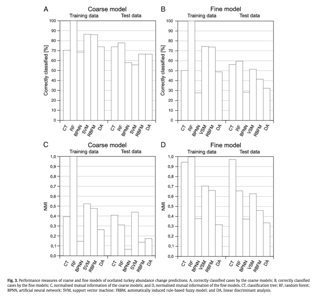
Machine learning methods have recently been adopted by ecologists to use in classification (eg. bioindicator identification, species distribution models, vegetation mapping) and there is an increasing amount of literature comparing the strengths and weaknesses of different machine learning techniques over a variety of applications. Kampichler et al add to this base of knowledge by comparing five machine learning techniques against the more conventional discriminant function analysis in their application to an analysis of abundance and distribution loss of the ocellated turkey (Meleagris ocellata) in the Yucatan Peninsula. They used data on turkey flock abundance (including absences) from the study area and 44 explanatory variables, including prior turkey abundance in local and regional cells, vegetation and land use types, and socio-demographic variables.

The techniques investigated were
– Classification trees (CT): uses a binary branching tree to describe the relationships between explanatory and predictor variables
– Random forests (RF): constructs many trees and then bags the trees to select the explanatory variables
– Back-propagation neural networks (BPNN): creates a network whose nodes are weighting by the training data
– Automatically induced fuzzy rule-based models (FRBM): processes variables based on algorithms using fuzzy logic
– Support vector machines (SVM): maps training data into an n-dimensional hyperplane and applies a kernel function to maximize seperation between the classes
– Discriminant analysis (DA): combines the explanatory variables linearly in an effort to “maximize the ratio between the separation of class means and within-class variance”

They compared the techniques based on their ability to correctly classify training and test data and using the normalized mutual information criterion, which is based on the confusion matrices and measures similarities between predictions and observations from 0 (random) to 1 (complete correspondence). In general, RF and CT performed the best, however the authors ranked CT first because of its high interpretability. An interesting point brought up is the fact that, in spite of the recent influx of machine learning in the scientific literature, most conservation decisions do not consider their results, most likely because of the lack of their interpretability and expertise needed to optimize the models. With this in mind, SVM, which performs relatively well, may not be the appropriate choice for conservation management because they are not well understood by ecologists lacking the proper mathematical training.

Screen Shot 2016-02-21 at 3.57.18 PM


Screen Shot 2016-02-21 at 3.57.45 PM

AUC: a misleading measure of the performance of predictive distribution models

Lobo, J. M., Jiménez-Valverde, A., & Real, R. (2008). AUC: a misleading measure of the performance of predictive distribution models. Global Ecology and Biogeography, 17(2), 145–151. http://doi.org/10.1111/j.1466-8238.2007.00358.x


With the increase in the use of predictive distribution models, especially with regards to species niche modeling, many are turning to the the area under the receiver operating characteristic curve (AUC) to assess the predictive accuracy of the models. Lobo et al have five main issues with the use of AUC in this manner. According to Lobo, AUC…

1) is insensitive to transformations of predicted probabilities, if ranks are preserved, meaning that models that are well fit may have poor discrimination and vice versa
2) summarizes test statistics in areas of extreme false-positive and –negative rates that researchers are rarely interested, leading the authors to suggest partial AUC
3) weights omission and commission the same. In the case of presence-absence data, false absences are more likely than false presence data, therefore their respective errors are not equal
4) plots do not describe the spatial distribution of errors, which would allow researchers to examine whether errors are spatially heterogeneous
5) does not accurately assess accuracy if the environmental range is larger than the geographical extent of presence data, as is the case for most SDM predictions

Additionally, AUC is often used to determine a ‘threshold’ probability of species distribution when converting a SDM to a binary, in spite of the fact that a ‘benefit’ of AUC is it is independent of the chosen threshold, and its corresponding subjectivity. The only instance in which the authors encourage use of AUC is in distinguishing between species whose distribution is more general (low AUC score) vs restricted. In order to combat the failings of AUC, Lobo et al suggest that sensitivity and specificity also be reported and that AUC only be used to compare models of the same species over an identical extent. I think another important point to include would be the quality of data. A cause of several of these problems is the bias of absence data in species distributions, and extra effort to combat this bias and ensure more complete presence-absence data sets would reduce the bias introduced by AUC.