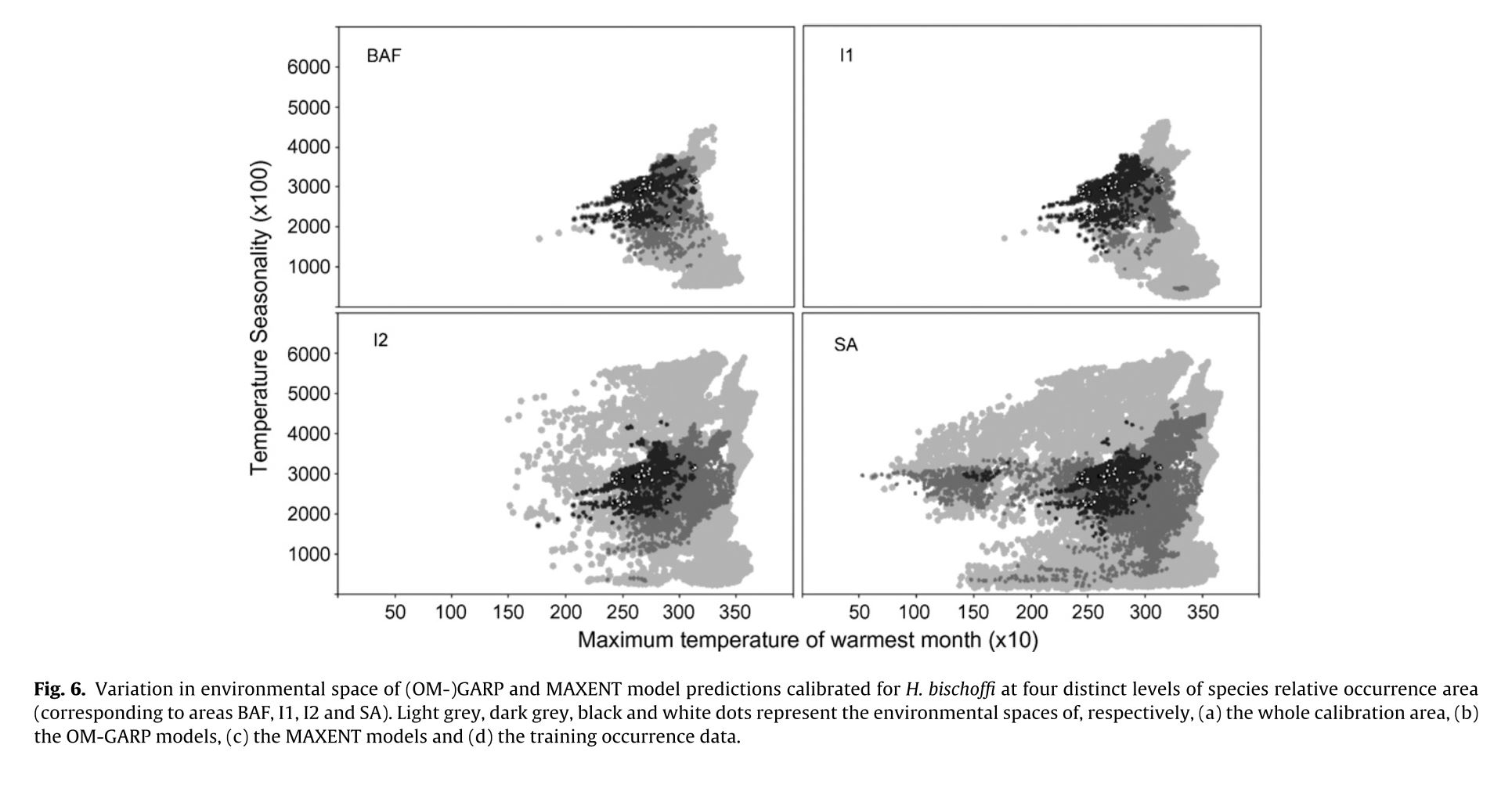
The authors set out to test the performance of five presence-only and presence-background SDM methods on sparsely recorded species in the neotropics. They use presence data on the common anuran Hypsiboas bischoffi to test the building of SDMs for species in the Brazilian Atlantic Forest (BAF). The models that they compare include: BIOCLIM (envelope based method in environmental space), DOMAIN (distance based method in environmental space), SVM (non-probabilistic statistical pattern recognition algorithms for estimating the boundary of a set), OM-GARP (a genetic algorithm which selects a set of rules that best predicts the distribution), and MAXENT. In addition to simply comparing the performance of these models in this region they also compare two alternative “calibration” domains for their models, the BAF and all of South America. “Calibration” domains defined the region from which pseudoabsence points were chosen for evaluation as well for training of presence-background models (OM-GARP and MAXENT). For those models that use pseudoabsence (OM-GARP and MAXENT) they examine how increasing calibration area (background) changes predictions in environmental space. These questions are relevant particularly in the Neotropics and more broadly because of the importance of modeling relatively unknown species with distributions of unidentified extents. Evaluation was performed using 5 random 75% training -25% testing partitions with 10 random pseudoabsences per occurrence point and assessed via AUC. Mean AUCs of models ranged from .77 (BIOCLIM/BAF) to .99 (MAXENT/SA). AUCs were always higher for models calibrated in SA than those in BAF. SVM had the highest AUC for BAF (.95) while MAXENT had the highest for SA (.99). BIOCLIM had the lowest AUC for both domains. The highest difference in predicted area for BAF vs. SA was OM-GARP’s. MAXENT was substantially more robust in its environmental predictions than OM-GARP to changes in extent of background area. As a result both SVM and MAXENT seem to be good choices for SDMs regardless of the unknown extent of the true distribution while OM-GARP may be a good option when the “calibration” area concurs relatively well with the extent of the “true” distribution. The most interesting results of this paper are the differences between OM-GARP and MAXENT in the way that their predictions are affected by a change in the extent of background points. This serves as yet another strong argument for MAXENT as a great choice model. Most of the remainder of the results seem to distill to the fact that evaluating in an increased area ought to lead to higher AUC because there are more obvious absence areas that are easily identified.
Category: Student summary
A Null-Model for Significance Testing of Presence-Only Species Distribution Models
Raes, N. and H. ter Steege (2007). “A null-model for significance testing of presence-only species distribution models.” Ecography 30(5): 727-736.
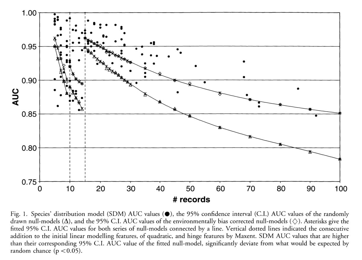
Validation of SDMs is both important and potentially difficult and problematic, especially in the case of presence-only data. Using pseudo-absence (background) points to calculate the AUC of trained models can create a number of problems, particularly that the maximum AUC is no longer 1 but rather 1-a/2 where a is the fraction of the landscape of interest genuinely covered by the species’ true distribution. As a result the interpretation of AUC values becomes muddied and typically “good” AUC values may not be what they seem. The authors propose a null model based approach to significance testing using “collection” localities, randomly drawn from the background, in equal number to the actual number of collection localities. This method relies, however, on the often unmet assumption that researchers have sampled all localities equally well. They propose to address this issue by drawing the random “collection” localities exclusively from the set of known collection localities. The authors illustrate this method using occurrences of the genus Shorea on the island Borneo and the SDM MaxEnt. They build both background based random null-models and null-models based on 1837 known collection localities for all plants across Borneo. Both of these types of null-models were used to construct a 95% confidence interval for AUC values such that AUCs outside of the interval implied that the model performed significantly differently from the random null model. 91% of species had a higher AUC than the random null-model CI, while only 61% had an AUC higher than the bias adjusted CI. In so doing, they show the importance of correcting for bias in your presence points when building null models, while recognizing that often researchers will not have an accessible set of nearly 2000 potential collection points to use for correcting their null-model. They suggest using distance to features such as roads, rivers, cities, and nature reserves, as a proxy for this data. They found that the AUCs of their true models and both null-models decreased with increasing number of presence points (and growing predicted range size) which they interpret to mean that as the unknown true distribution of the species increases only the maximum AUC decreases and not the actual predictive ability of models. Though the concept of null-model based hypothesis testing has been used previously in SDM and elsewhere of course as well, the addition of the bias-corrected null model seems valuable for effective evaluation. It does ignore, however, the fact that the actual predictive accuracy of a given model will be affected by bias in the presence data. This method, though, may make our AUC evaluations more fair and accurate and so seems worth further study.
Big Data, new epistemologies and paradigm shifts
Kitchin, R., 2014. Big Data, new epistemologies and paradigm shifts. Big Data & Society, 1(1), p.2053951714528481.
This article argues that the explosion in the production of Big Data and the advent of new science epistemologies where questions are born from the data rather than testing a theory by analyzing data has far-reaching consequences to how research is conducted. One section evaluates whether the scientific method is rendered obsolete with the production of Big Data. Instead of making educated guesses about systems, constructing hypotheses and models, and testing them with data-based experiments, scientists can now find patterns in data without any mechanistic explanation at all. But in some fields, this doesn’t really matter. For example, in online retail stores Person A might be known to like item A and most people that like item A also like item B. In this situation, the mechanism does not really matter for the retail company to sell more items. Thus, mining the entire population’s behavior for prediction trumps explanation for the retail markets. But the result is an analysis that ignores important effects of culture, politics, policy, etc. So expanding these ideas to the field of biology might include a bioinformatist that view the complexity of biology in a much different way that an experimental molecular biologist. To an informatist, data can be interpreted free of context and domain-specific expertise but it might be low on logical interpretation.
It seems to me that the majority of ecologists are aware of the concerns that Kitchin raises and would probably side with him on most points, especially when thinking about mechanisms causing patterns rather than settling with knowing the correlations that coincide with them. Nevertheless, I think it was a good read and one that helped me contextualize some disagreements between Big Data and production of new science.
A climate of uncertainty: accounting for error in climate variables for species distribution models
Stoklosa, J. et al., 2015. A climate of uncertainty: accounting for error in climate variables for species distribution models R. B. O’Hara, ed. Methods in Ecology and Evolution, 6(4), pp.412–423.
Climate variables used in species distribution models are estimates of true spatial climate and are therefore subject to uncertainty. The uncertainty itself can have spatial structure, further complicating consistency of estimates. The authors of this study chose to use PRISM (parameter elevation relationships on independent slopes models) to obtain estimates of climate uncertainty. To do this, they construct grids of approximately 800x800m size and use these estimates as an upper bound to prediction error variance of the climate model.
They also wanted to understand what happens if this uncertainty is ignored. Other fields, such as engineering and medicine, use measurement error models that allow uncertainty in explanatory variables (errors-in-variable) but can sometimes lead to biased estimates. This study used hierarchical modeling and simulation extrapolation to account for errors in explanatory variables. Wren presence/absence data (n=1048 data points) was obtained from birders at several points along a transect of the Eastern US. They test these methods on the Carolina wren in the US and on simulated species to look at how well GLMs predict and project to new scenarios when prediction error is ignored versus when it is accounted for. The main effect of ignoring uncertainty in climate variables was an increase in bias and a decrease in power as the error increases. These methods seem likely to be useful in situations where a species is patchily distributed or in environments that are spatially autocorrelated.
Using species distribution modeling to assess factors that determine the distribution of two parapatric howlers (Alouatta spp.) in South America.
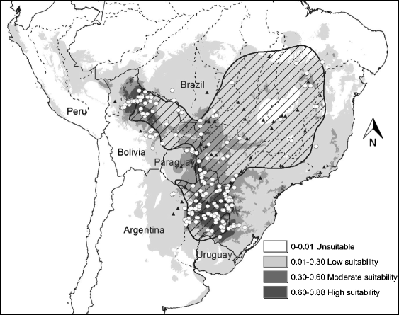
The authors use MaxEnt to model the distribution of two species of howlers (Alouatta caraya and Alouatta guariba clamitans). The data was collected from four sources: museum species from GBIF, publications, unpublished records, and field survey from 3/2008 to 11/2009. The full set of bioclimatic variables consisted of 19 variables. The model for Alouatta caraya used 196 presence points and 8 of the 19 climatic variables. The model for A. guariba clamitans used 74 presence points and 13 climatic variables.
Habitat suitability (low, moderate, high) categorized the resulted of the predicted areas. In addition, the models were evaluated using AUC. Both the models provided a wider distribution than currently estimated. The results of the model for Alouatta caraya had a broader range and a variety of temperatures with Temperature Annual Range as the most influential to the distribution.
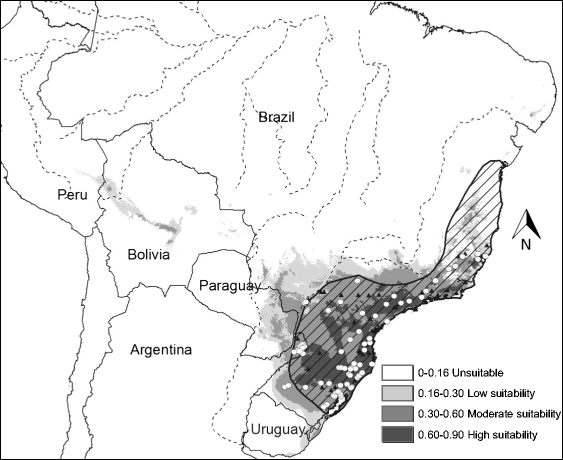
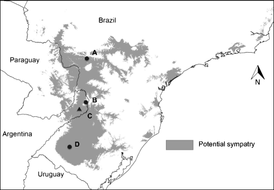
For A. guariba clamitans the species was more contrained to rainy areas of the forest with high altitudes and low minimum temperatures. This species was most influenced by Mean Temperature of the Coldest Quarter.
There was also a region of overlap between the species which suggests (as positioned by the authors) a difference in foundational niches of the species. This overlap could result in hybridization potentially limiting the overlap. In addition, the authors posit that the overlap zone could be maintained by the Parana River.
Holzmann, I., Agostini, I., DeMatteo, K., Areta, J. I., Merino, M. L. & Di Bitetti, M. S. 2015 Using species distribution modeling to assess factors that determine the distribution of two parapatric howlers (Alouatta spp.) in South America. Int. J. Primatol. 36, 18–32.
A null-model for significance testing of presence-only species distribution models
Findings from Olden 2002, Predictive models of fish species distributions: a note on proper validation and chance predictions, points to that fact that there is a critical need for a method to evaluate whether or not SDM predictions would differ from what would be expected from chance alone. This paper provides a null-model in an attempt to address the ideas outlined in Olden 2002. Researchers point out that a major drawback to AUC in pseudo-absence approaches is that the AUC value indicating a perfect fit is not 1 but instead 1-a/2. Where a is the fraction of the geographical area of interested covered by a species’ true distribution which is typically an unknown quantity.
Developing the null model for evaluating AUC estimates.
- Determine the AUC value of the real SDM from provided data.
- Generate a null model by randomly collecting localities without replacement from the target species supposed distribution area.
- The number drawn is equal to the number of occurrence points within the data set.
- Repeat this process until you are able to draw a stable frequency histogram of AUC values.
- Compare the expected real AUC value against the histogram of null based AUC values and determine the probability value. Use a one sided 95% confidence interval to evaluate your real AUC value.
One potential benefit of the proposed method is that it doesn’t require the researcher to split their data set into training and test data sets. However, major assumption is that all occurrence localities are sampled equally. If this assumption is not met then the developed null model may be biased in favor of the heavily sample locations.
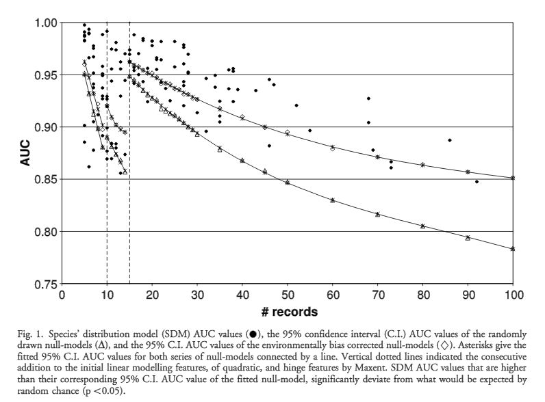
Researchers demonstrated the effectiveness of their null-model by way of case study using the occurrence records of plants from the genus Shorea. The SDM selected was MaxENT with a list of environmental data sources. Results are able to demonstrate how null models that better correct for environmental bias often produce lower AUC values than their traditional MaxENT counterparts (Fig. 1).
The use of the area under the ROC curve in the evaluation of machine learning algorithms
The author of this paper puts forth the idea that evaluation of machine learning algorithms can be evaluated by employing receiver operator curves and determining the area under said curves. The problem outlined in this paper is how to effectively evaluate the performance of a model that is trained on provided examples. In this paper the author introduces a technique for estimating the area of the curve, and demonstrates how effective the proposed technique is by using data from six case studies.
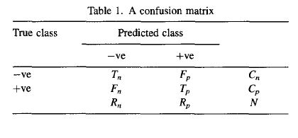
ROC curves are related to the confusion matrix table.
In the confusion table Tn represents the True negative rate, Fp represents the false positive, Fn represents the false negative rate, and Tp represents the True positive rate. Summing across the rows we have Cn which is the True negative number, CP the True positive number. For column sums we have the Predictive negative (Rn) and Predicted positives (Rp). From these numbers we can evaluate the classifier with the following summary statistics: accuracy, sensitivity, specificity, positive predictive value and negative predictive value.
Bradely points out that all of the measures mentioned above are only valid for a specific threshold point, and that estimating the area under the curve from ROC curves would overcome this drawback. Another technique presented here is how to determine the standard error for AUC estimates.
The datasets considered in this paper revolve around health outcome diagnosis with two output classes. Machine learning methods evaluated are the following: quadratic discriminant function, multiscale classifier, k-nearest neighbor, C4.5, perceptron, and multi-layer perceptron.
A key finding of this paper is demonstrating how AUC estimates are similar in their application to the Wilcoxon rank statistic (Section 9.3.1). For a more indepth summary of the results refer to the figures provided within the manuscript.
Do Hypervolumes Have Holes?
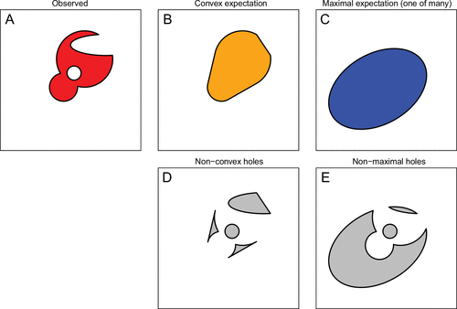
A ecological niche can be defined (as by Hutchinson 1957) as the n-dimensional hypervolume that describes the environment allowing the species to exist. The hypervolume concept has been used to describe not only the niche of a species but also trait distributions of communities. Hypervolumes, as described by Blonder, can be convex describing the fundamental niche of a species where the boundaries of the area only have upper and lower limits. These can also be maximal where the boundaries are the available space representing the potential niche (the relationship between convex and maximal hypervolume concept relates to Drake 2015, Range Bagging). However, observed hyper volumes may have holes. These holes may be a result of not considered ecological or evolutionary processes of the species. Blonder developed an algorithm to detect holes within a hypervolume.
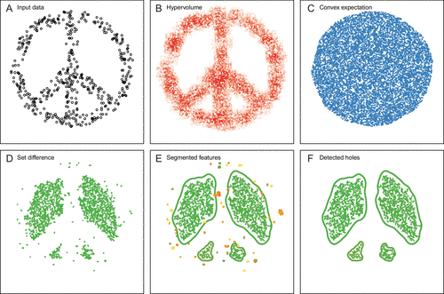
The Algorithm (an outline, featured image):
- Obtain input data in the form of an m x n matrix with m data points and n continuous, environmental variables.
- Compute a hypervolume H that encloses all data points using the hypervolume R function. The produces a stochastic geometry representation of the hypervolume, R_H
- Compute a hypervolume B with stochastic geometry representation R_B for the baseline expectation.
- Perform a stochastic geometry set difference S=R_B\R_H (all the points that are contained the baseline expectation (convex hull without holes) and the hypervolume with holes).
- Segment holes from the set difference.
- Remove small holes.
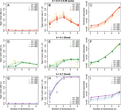
Using this algorithm with simulated data, Bolder found that Type I error rate (say there is a hole when there is not one) generally does not increase with data dimensionality. However, Type II error rate (say there is not a hole where there is one) does increase with dimensions, up to 100%. Also, increases in dimensions results in an exponential increase in runtime.
Blonder, B. 2016 Do Hypervolumes Have Holes? Am. Nat. 187, E93–E105. (doi:10.1086/685444)
The effect of sample size and species characteristics on performance of different species distribution modeling methods
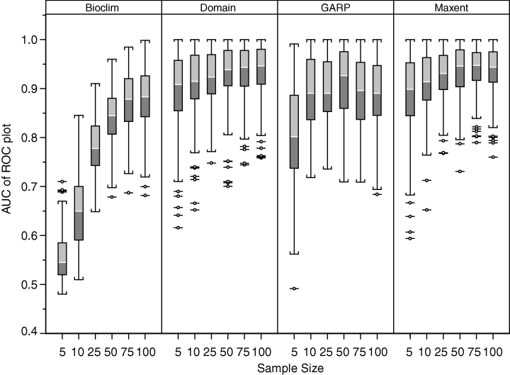
Species, especially those of interest to conservationists, often have limited to rare occurrence data. This “sparseness” of the occurrence data poses problems with developing accurate distribution models/predictions. Previous studies have examined the effect of sample size on the accuracy of these SDMs; however, the sample size of individual species has not been investigated. Individual species characteristics, such as range size, may impact the accuracy of the models. The authors examine the impact of sample size on model accuracy for 18 taxa (California taxa) using 4 modeling methods using presence only data.
Of the methods used, MaxEnt provided the most useful results even as small sample sizes (5, 10, 25, of the maximum 150). The Domain and GARP performed reasonably well with the small sample sizes. However, Bioclim performed with worst. They also point out that multiple measures of model accuracy, not just AUC, are needed to determine the performance. In terms of species characteristics on model performance, species with smaller ranges, both geographical and environmental, provided greater accuracy in the models. The authors then highlight that these models should be used by conservationists to estimate rare species distributions.
Hernández, P. A., Graham, C. H., Master, L. L. & Albert, D. L. 2006 The effect of sample size and species characteristics on performance of different species distribution modeling methods. Ecography (Cop.). 29, 773–785. (doi:DOI 10.1111/j.0906-7590.2006.04700.x)
Machine Learning Methods Without Tears: A Primer for Ecologist
Olden, Julian D., Joshua J. Lawler, and N. LeRoy Poff. “Machine learning methods without tears: a primer for ecologists.” The Quarterly review of biology 83.2 (2008): 171-193.
Overview
This paper was designed to help facilitate the application of machine learning techniques into the field of ecology. Authors posit that despite the advantages of machine learning techniques, ecologists have been slow in integrating these methods into their research due to lack of familiarity. It is the intent of this paper to provide background information on three categories of machine learning and examples of use in the ecological literature.
Classification and Regression Trees (Cart)
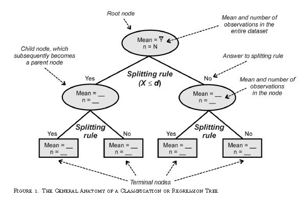
Carts can are a form of binary recursive partitioning where classification is based upon making splits within the provided dataset. The three basics of a cart algorithm involve tree building, stopping the tree building, and tree pruning and optimal selection. One of the biggest strengths of carts compared to other machine learning methods is that they’re relatively easy to interpret. One weakness is that decision trees are typically unstable.
Artificial Neural Networks
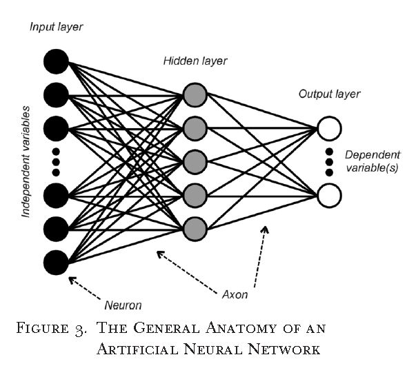
Also known as multilayer perceptrons, artificial neural networks are considered to be the universal approximations of any continuous function. Neural networks are comprised of three primary components, input layer (independent variables), While there are different types of neural networks, this paper presented the feed forward network. In a feed forward network each neuron of the previous(layer) is connected to all neurons of the next layer via axons. Connections are weighted by an activation energy function. A core strength of neural networks is that many of the underlying features can be modified to suite the research task at hand. While a weakness to neural networks would be that model performance can be sensitive to random initial conditions (weights).
Genetic Algorithm or Genetic Programming
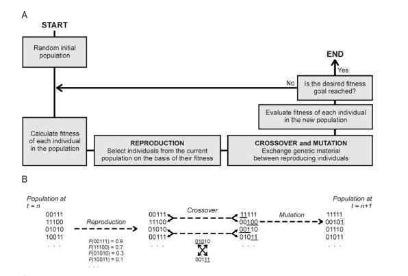
The conceptual idea behind genetic programing is that algorithms operate in a population of competing solutions to one problem, and the best solution evolves over time. Solutions are comprised of chromosomes and the chromosomes are comprised of “genes”. Genetic algorithms are strong in handling stochastic optimization procedures, but are more susceptible to model overfitting.
Conclusion
The purpose of this paper was to provide ecologist and biologist with a basic introduction to machine learning techniques and how they can be applied to ecological problems. Authors stress that while machine learning techniques can be a major boon in ecological research, machine learning will not be a end all solution to problems facing ecology. Rather, machine learning approaches should be considered an alternative to problems in massaging messy data into classical statistical models.