Biotic interactions boost spatial models of species richness

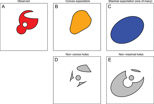
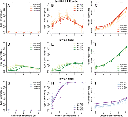
Integrating biotic interactions into the framework of species richness models has been a suggested to improve the performance of both species distribution models.  The authors seek to use biotic variables in two species richness modeling frameworks.  Stacked species distribution models (SSDM) fit separate species distribution models then blindly stacks the results of the predicted occurrences to calculate the species richness.  The macroecological models (MEM) do not use the information provided by species identity and community composition to estimate the species number using environmental conditions.  This model assumes species richness is limited by environmental conditions. Using these two models, three different groups of taxa (vascular plants, bryophytes, and lichens) used to examine the effect of integrating biotic variables.

When comparing the results of the models using biotic interactions to models with only climatic and abiotic, biotic models performed consistently better.  Both modeling frameworks and all taxonomic groups using biotic interactions had a lower bias and increased predictive power. These results highlight the importance of using biotic predictor variables in not only species richness models but also single species distribution models.

Mod, H. K., le Roux, P. C., Guisan, A. & Luoto, M. 2015 Biotic interactions boost spatial models of species richness. Ecography (Cop.). 38, 913–921.

The role of biotic interactions in shaping distributions and realized assemblages of species: implications for species distribution modeling

As with Mod (2015), the integration of biotic interactions/variables into species distribution models is of interest.  It is already know that at small, local scales biotic interactions influence the distribution of species.  However, in order to integrate these interactions at a larger scale and in the future, a better understanding of how these interactions have influenced the species historically and dispersal.  The authors provide a review using studies involving species ranges, functional groups, and patterns of species richness.

The authors find that the biotic interactions have shaped the distribution of species beyond the local extent (10 km^2). The authors then suggest and review some ways to integrate biotic interactions within species distribution models.  These include using pairwise dependencies, using integrative predictors, and lastly hybridizing the models with dynamic models.

However, there are some problems with integrating these.  One possible problem is that species interactions may not be constant in time and space.  All the integrated models would assume that the interaction would be static between species. Any changes in species composition may affect these interactions through time and also space.  The authors close by calling for better data collection across scales and along environmental gradients.

Wisz, M. S. et al. 2013 The role of biotic interactions in shaping distributions and realised assemblages of species: implications for species distribution modelling. Biol. Rev. 88, 15–30.

Using species distribution modeling to delineate the botanical richness patterns and phytogeographical regions of China

Due to the recent archiving and georeferencing of plant specimen collected over the past century, the distribution modeling of these species is now easily possible. The authors modeled the distribution of 6,828 species and determined the biological richness of areas in China.  In addition, they also investigated the drivers of the richness in the areas.

To prediction the distribution of the species, they used MaxEnt.  To analyze regions of species richness, they used ordination and Getis-Ord Gi* statistics finding hotspots of species richness. These also allowed them to determine the drivers of species richness and hotspots.

srep22400-f1


Of the predictors used, annual precipitation and temperature stability provided a major role in the observed species diversity.  However, when looking at the different regions, there were different drivers:

  • SE – annual precipitation
  • SW – topographic & temperature stability
  • NW – water deficit
  • NE – temperature instability


srep22400-f3

Fifteen uncorrelated variables plotted as predictors of environmental turnover calculated for 6560 woody species. Vectors are displayed only for the highly significant variables (P < 0.001) inferred from non-metric multidimensional scaling (NMDS) ordination. TAR: Temperature Annual Rang.

Zhang, M.-G., Slik, J. W. F. & Ma, K.-P. 2016 Using species distribution modeling to delineate the botanical richness patterns and phytogeographical regions of China. Sci. Rep. 6.

Modeling hotspots of the two dominant Rift Valley fever vectors (Aedes vegans and Culex poicilipes) in Barkédji, Sénégal

In relation to Mosomtai et al. (2016) (see Association of ecological factors with Rift Valley fever occurrence and mapping of risk zones in Kenya) these authors predict the distribution of the two vectors for Rift Valley fever (RVF).  Previous studies have looked at disease risk by finding areas with high vectors pressure or virus activity.  Here the authors investigate the impact of climate and environment on the presence of Aedes vegans and Culex poicilipes  (the two primary vectors of RFV).

13071_2016_1399_Fig1_HTML

Mosquito data was gathered from the Barkedji village (Ferlo area) during 2005 to 2006 across 79 sites.  After collecting the data, the Getis-Ord statistic was calculated to determine hotspots (adult mosquito abundance clusters).  The Getis-Ord Gi* measures the spatial clustering by identifying hotspots with a higher magnitude than expected from random chance. To deal with spatial autocorrelation, generalized linear mixed effect models were used.  The response/dependent variable was the calculated Getis-Ord Gi* of the hotspots.  The predictor/independent variables were rainfall, relative humidity, max and min temperature, NDVI, and distance from nearest pond.

13071_2016_1399_Fig6_HTML

For the Culex species, drops in the minimum temperature allows for an increase the occurrence of hotspots.  For the Aedes species, there is a negative relationship with relative humidity, max and min temperatures and hotspot occurrence. For both species, the distance to the nearest pond increases the occurrence of a hotspot. The authors close the paper by commenting that these models and understanding what promotes the occurrence of hotspots can lead to better vector control in the area.

Talla, C., Diallo, D., Dia, I., Ba, Y., Ndione, J.-A., Morse, A. P., Diop, A. & Diallo, M. 2016 Modelling hotspots of the two dominant Rift Valley fever vectors (Aedes vexans and Culex poicilipes) in Barkédji, Sénégal. Parasit. Vectors 9, 1.

Association of ecological factors with Rift Valley fever occurrence and mapping of risk zones in Kenya

The focus of the paper is to create a spatial risk map for Rift Valley Fever (RVF) using ecological and environmental variables.  RVF is a mosquito borne infection in vertebrates.  There are typically outbreak of the disease after periods of rainfall and high temperatures.  These outbreaks occur in 5 to 15 year intervals with flareups occurring between.  Previous studies that have looked at RVF occurrences have not used explicit ecological factors in their models.  Here the authors use explicit factors to map the risk of RVF in Kenya.  Areas of risk were defined as areas that were able to support the vectors in habitat suitability and population dynamics.

The authors use a generalized linear model to relate the ecological predictors to the occurrence data.  For the predictor variables, animal/livestock density, elevation, season length, small vegetation integral, soil ratio, and two principle components of evapotranspiration (PC1_ET and PC2_ET) were used.

gr5

Of the predictors, livestock density, small vegetation integral, and PC2_ET were the most significant variables.  In Kenya, the Tana River, Garissa, Isiolo and Lamu were the areas of highest risk. The authors also close by suggesting the integration of livestock movement and density along with the vegetation measurements into early warning systems.

Mosomtai, G., Evander, M., Sandström, P., Ahlm, C., Sang, R., Hassan, O. A., Affognon, H. & Landmann, T. 2016 Association of ecological factors with Rift Valley fever occurrence and mapping of risk zones in Kenya. Int. J. Infect. Dis. 46, 49–55.


Species distribution models and ecological suitability analysis of potential tick vectors of Lyme Disease in Mexico

Lyme disease, a a tick-borne disease caused by Borrelia burgdorferi,  has had an increasing number of cases occur in Mexico.  While the disease is rare in the Southern United States, it has been found to occur in Northern and Mid-Western US and Europe.  The authors investigate the distribution of potential tick vectors (ten Ixodoes spp. and Amblyomma cajennense [inclusion of this species as a vector is through personal communication]) in Mexico.

Occurrence data of the ticks was collected from prior publications and field surveys.  However, the occurrence data for ticks in Texas and Mexico was too sparse to do the models independently.  While the data used was collected in both Mexico and Texas, the authors only present the results for Mexico.  Environmental data was collected from WorldClim.  The distribution model used was MaxEnt and the trained for the Amblyomma cajennense  and the ten Ixodoes as a group.

JTM2012-959101.003

From the results, there is spatial non concordance between the species.  Amblyomma cajennense  was mainly predicted to occur in mangrove and marsh regions at lower altitudes along the coast (red region).  The Ixodoes group are mainly found in oak and pine-oak forests.  These results highlight that if a species in the Ixodoes group is capable of transmitting the pathogen then the areas of highest risk are at high-altitude low temperature areas (which helps explain why Lyme disease is so rare in the southern US, high temperatures). However, if it is true that Amblyomma cajennense is capable of maintaining the pathogen in reservoir hosts, then the region extends  eastern lowlands of Mexico.

Illoldi-Rangel, P. et al. 2012 Species distribution models and ecological suitability analysis for potential tick vectors of Lyme disease in Mexico. J. Trop. Med. 2012.

Geographic distribution of Chagas disease vectors in Brazil based on ecological niche modeling

Chugs disease is caused by Trypanosome cruzi parasite which is primarily transmitted through kissing bugs (triatomines).  While control measures have been implemented to help control the domestic vector population in Brazil and have shown to be effective in reducing disease occurrence, there are still reported cases of the disease transmitted from the native vectors. These occurrences can be there result of sylvatic vectors invading households, contamination of food, or domestic/peridomestic vectors.  The authors investigate the distribution of 62 Brazilian species of the vectors.

MaxEnt was used to model the distributions.  Occurrence data for the species was collected from multiple sources including Brazilian State Health Departments. Environmental data was used from two datasets: multitemporal remotely sensed imagery (Advanced Very High Resolution Radiometer satellite) and climatic variables (WorldClim). Of the species modeled, P. geniculatus and P. megistus had the largest/broadest distribution.

705326.fig.008

Species diversity map, darker red regions have higher predicted cooccurring species.

The most favored regions for the vectors are the Cerrado and Caatinga, the diagonal open areas in eastern South America.  The results also highlight the nowhere in Brazil is Chagas risk small but some regions are of higher risk than others. Also, the current distribution of T. infestans (the domestic vector) shows the impact and effectiveness of the control measures.

Gurgel-Gonçalves, R., Galvao, C., Costa, J. & Peterson, A. T. 2012 Geographic distribution of Chagas disease vectors in Brazil based on ecological niche modeling. J. Trop. Med. 2012.

Using species distribution modeling to assess factors that determine the distribution of two parapatric howlers (Alouatta spp.) in South America.

The authors use MaxEnt to model the distribution of two species of howlers (Alouatta caraya and Alouatta guariba clamitans).  The data was collected from four sources: museum species from GBIF, publications, unpublished records, and field survey from 3/2008 to 11/2009.  The full set of bioclimatic variables consisted of 19 variables.  The model for Alouatta caraya used 196 presence points and 8 of the 19 climatic variables.  The model for A. guariba clamitans used 74 presence points and 13 climatic variables.

10764_2014_9805_Fig2_HTML
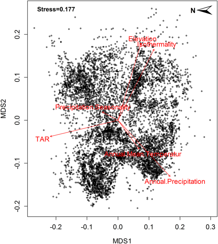
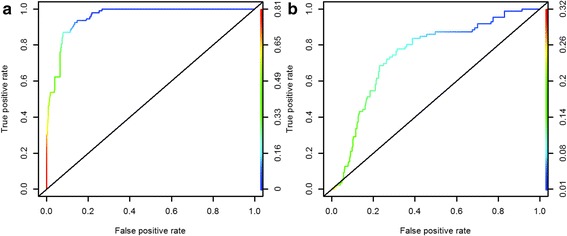
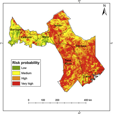
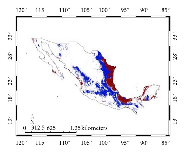
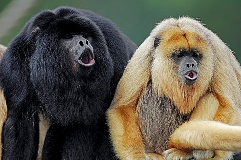
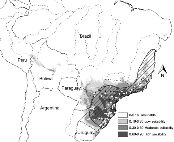
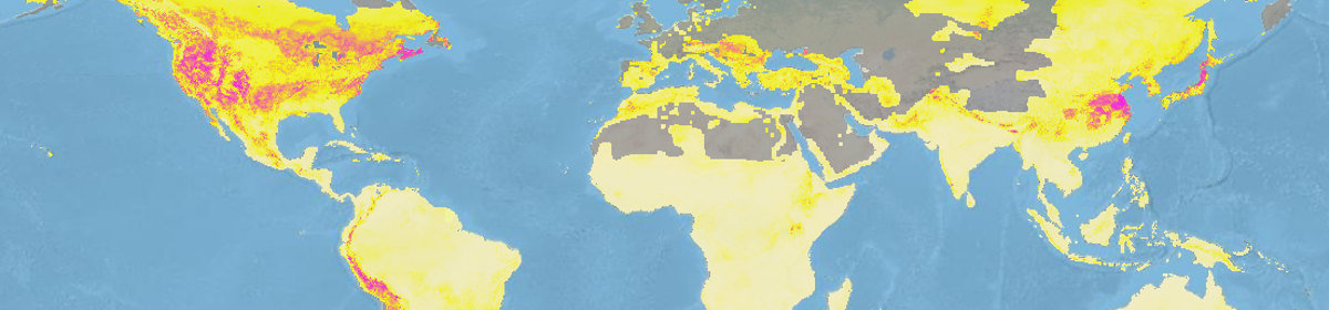
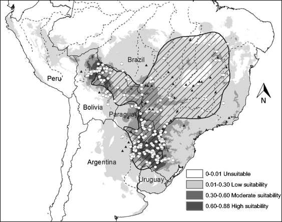
Habitat suitability (low, moderate, high) categorized the resulted of the predicted areas.  In addition, the models were evaluated using AUC. Both the models provided a wider distribution than currently estimated. The results of the model for Alouatta caraya had a broader range and a variety of temperatures with Temperature Annual Range as the most influential to the distribution.

10764_2014_9805_Fig3_HTML

For A. guariba clamitans the species was more contrained to rainy areas of the forest with high altitudes and low minimum temperatures. This species was most influenced by Mean Temperature of the Coldest Quarter.

10764_2014_9805_Fig4_HTML
There was also a region of overlap between the species which suggests (as positioned by the authors) a difference in foundational niches of the species. This overlap could result in hybridization potentially limiting the overlap.  In addition, the authors posit that the overlap zone could be maintained by the Parana River.

Holzmann, I., Agostini, I., DeMatteo, K., Areta, J. I., Merino, M. L. & Di Bitetti, M. S. 2015 Using species distribution modeling to assess factors that determine the distribution of two parapatric howlers (Alouatta spp.) in South America. Int. J. Primatol. 36, 18–32.

Empirical evidence for source-sink population: a review on occurrence, assessments, and implications

The paper provides a review and synthesis examining the occurrence of source and sink populations in the literature.  Pullman (1988) stated that sink habitats would need inputs from nearby sources to persist in the landscape. As the need for conservation planning increases, a better understanding of what may affect the presence of source and sink habitats is crucial. Prior to performing the analysis, the authors provide systematic and biological predictions about what may influence source and sink population occurrence.

Methodological:

  1. There will be less evidence for source populations then sink population.
    1. The authors were correct in this prediction there was more evidence for sink populations across taxa (however, this finding was not significant, p=0.059).

brv12195-fig-0002 brv12195-fig-0002

Black bars represent source populations. Grey bars are sink populations.

  1. The spatial scale of the studies will affect the detection/occurance of source and sink populations.
    • Was not supported.
  2. When several, i.e. more than a few(?), local populations are considered, there will be more evidence for source populations.
    • Was not supported.
    • The authors comment that more demographic data should be record when examining populations (i.e. fecundity/mortality, immigration/emmigration).

Biological

  1. More sources are expected when the local population is stable or increasing. Sinks when the local population is decreasing.
    • Was not supported.
  2. Sources are expected in resident species rather than migratory.
    • Was not supported.
  3. Low-dispersal ability species are expected to have more sources than high dispersal ability species. Also, high dispersing species are expected to have more sinks than limited dispersal species.
    • Was not supported.
  4. Well-connected local populations are expected to have more sources.
    • The prediction was supported, local populations that were well-connected were more likely to have sources. Immigration between may prevent stochastic/demographic extinction of patches.
  5. Specialist species, that can only utilize a limited range of environmental conditions, are expected to have more sink habitats.
    • Was not supported
  6. Sources were expected to occur more often in the middle of species ranges, with sinks occurring on the edge.
    • Was not supported.

Furrer, R. D. & Pasinelli, G. 2015 Empirical evidence for source–sink populations: a review on occurrence, assessments and implications. Biol. Rev.

Do Hypervolumes Have Holes?

A ecological niche can be defined (as by Hutchinson 1957) as the n-dimensional hypervolume that describes the environment allowing the species to exist.   The hypervolume concept has been used to describe not only the niche of a species but also trait distributions of communities. Hypervolumes, as described by Blonder, can be convex describing the fundamental niche of a species where the boundaries of the area only have upper and lower limits.  These can also be maximal where the boundaries are the available space representing the potential niche (the relationship between convex and maximal hypervolume concept relates to Drake 2015, Range Bagging). However, observed hyper volumes may have holes.  These holes may be a result of not considered ecological or evolutionary processes of the species. Blonder developed an algorithm to detect holes within a hypervolume.

fg1

The Algorithm (an outline, featured image):

  1. Obtain input data in the form of an m x n matrix with m data points and n continuous, environmental variables.
  2. Compute a hypervolume H that encloses all data points using the hypervolume R function.  The produces a stochastic geometry representation of the hypervolume, R_H
  3. Compute a hypervolume B with stochastic geometry representation R_B for the baseline expectation.
  4. Perform a stochastic geometry set difference S=R_B\R_H (all the points that are contained the baseline expectation (convex hull without holes) and the hypervolume with holes).
  5. Segment holes from the set difference.
  6. Remove small holes.

Using this algorithm with simulated data, Bolder found that Type I error rate (say there is a hole when there is not one) generally does not increase with data dimensionality. However, Type II error rate (say there is not a hole where there is one) does increase with dimensions, up to 100%.  Also, increases in dimensions results in an exponential increase in runtime.

fg4

Blonder, B. 2016 Do Hypervolumes Have Holes? Am. Nat. 187, E93–E105. (doi:10.1086/685444)