The ability of climate envelope models to predict the effect of climate change on species distributions

Hijmans, Robert J., and Catherine H. Graham. “The ability of climate envelope models to predict the effect of climate change on species distributions.” Global change biology 12.12 (2006): 2272-2281.

DOI: 10.1111/j.1365-2486.2006.01256.x

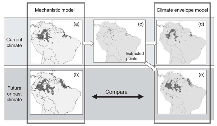
Hijman and Grahams objective was to evaluate whether Climate Envelope Models (CEM) are as successful in predicting species distribution under future climate change scenarios as it is in predicting current species distribution. They evaluated CEM ability by comparing CEM predictions with predictions obtained from Mechanistic Models (MM, which are based on an understanding of species physiology while CEMs use known geographic locations of a species to infer on their environmental requirements). They evaluated data from 100 plant species for past, current, and future distributions, by comparing MM results with four different CEM that covered a range of statistical approaches: BioClim, Domain, GAM, and Maxent and used range size, overlap index, false positive rate, and false negative rate to determine how well species distribution with CEM corresponds with MM (Generally illustrated in Fig. 1). The concern is that some CEMs may be unsuitable to predict species ranges under future climate because 1) cannot be tested using independent model training and testing data sets (i.e. no observed data for future scenarios and 2) a statistical model in which the inferred environmental requirements may not be suitable for truly classifying suitable vs. unsuitable environments. Hijmans suggests to compare results from CEM with MM, because using MM will model species distribution using physiology independent of climate. However, the only problem with MM is that physiology data is not always easy to gather. There was considerable variation between CEM and ability to reproduce the predictions from MM. Maxent and GAM provided good estimates for range shift with climate change. Domain underestimated range size. Bioclim underestimates future ranges, so would be considered a conservative approach, for example for reserve planning. Don’t even go with Domain, because it was considered too sensitive to the number of environmental variables used to predict species distribution. They came to the conclusion that some CEMs are reasonably good at predicting species dristributions under a climate change scenario.

In this paper, to assess species distribution changes in response to climate change, nonclimatic effects were eliminated. This is not very realistic however, because species distributions is likely influenced by both biotic and abiotic factors. It would be interesting to take biotic factors into account, because most likely species interactions with one another may be indirectly linked to changes in distribution driven by abiotic factors (one would persist and the other may not?). Also, applying this to vertebrate data, and even more interestingly, a migrating species, would be a great next step for using CEM to predict future species distribution.

(Figure caption: Approach used to evaluate the ability of climate envelope models to predict species distributions under different climates. A mechanistic model is used to predict the potential distribution for a species under current (a) and future (or past) (b) conditions (light gray = not suitable, dark gray = suitable). Points are extracted randomly from the area deemed currently suitable for the species (c). These points are used in the climate envelope model for current (d) and future (e) conditions. The statistical model is evaluated through a comparison of (b) and (e).)



Cross-validation of species distribution models: removing spatial sorting bias and calibration with a null model

Hijmans, R.J., 2012. Cross-validation of species distribution models: removing sorting bias and calibration with a null model. EcologyLink to paper

Spatial sampling biases, or the observation that testing presence points tend to be closer in space than do testing absence points (and the credibility of cross-validation for assessing model accuracy) remain large issues for SDMs. Hijmans (2012) evaluates two different ways of selecting testing-presence data and two ways of selecting testing-absence data in order to better understand how spatial sampling biases and cross-validation may lead to inflated confidence in SDMs. Indeed he found that a null model, based solely on distance to nearest presence point, performed just as well (.69) as Bioclim (.64) and Maxent (.73). This suggests that it can be difficult to directly interpret uncallibrated cross-validation results (as is seen in most studies using SDMs) and that calilibrating with a null model could lead to more accurate predictions. This study calls into question many results from SDMs, especially those using data that is inherently clumpy (e.g. museum records). I think this is an especially open area for research with questions such as: How can knowledge of a species biology be used to pre-process (filter) species occurrence data before being input into SDMs? Or how does clumpiness of species occurrence data affect predictability of species range?

The Crucial role of the accessible area in ecological niche modeling and species distribution modeling

Barve, Narayani, et al. “The crucial role of the accessible area in ecological niche modeling and species distribution modeling.” Ecological Modelling 222.11 (2011): 1810-1819.

doi:10.1016/j.ecolmodel.2011.02.011

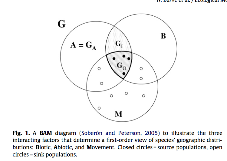
Conceptual biases remain little explored in broad-scale ecological niche modeling and species distribution modeling. Species can respond environment in diversy ways: ecological niches may evolve or remain conserved. According to the conceptions in the BAM diagram (Fig 1), the region where species can be found is the intersection of A (environmental factors with values not dependent on species population dynamics, B (sets of variables that are dependent on species population), and M (regions that are accessible by the species but are unrelated with A). Region M depends on opportunities for and constraints on movements of species and is often not included in modeling efforts. Barve et. al. examined the conceptual and empirical reasons behind the choice of study area extent and presented 3 approaches for M estimation: 1. Biotic regions. Regions within which a species is known to occur; 2. Niche-model-based regions. The reconstructed historical distributions of species from models based on their current ecological niche characteristics; and 3. Full dynamic dispersal model, which takes into consideration exolicitly the spatially path-dependent nature of effects of environmental change. They asserted that the accessible area over relevant time periods are the most appropriate for model development, testing, and comparison. Although Barye et. al. emphasized on estimating the set of areas that species were sampled for niche modeling, this idea also has implications for biogeography, macrogeography, and phylogeography.Screen Shot 2016-03-02 at 12.21.23 PM

Data prevalence matters when assessing species’ responses using data-driven species distribution models

Fukuda, S. & De Baets, B., 2016. Data prevalence matters when assessing species’ responses using data-driven species distribution models. Ecological Informatics, 32, pp.69–78.  link to paper

The accuracy of SDMs is highly dependent on the quality and quantity of data used such as size (i.e. the number of data points in a data set) and data prevalence (i.e. the proportion of presences in a data set) matter for SDM accuracy. Fukuda et al. (2016) investigated this observation by simulating nineteen sets of virtual species data in real habitat conditions (using field observations) and hypothetical habitat suitability curves under four conditions. Then they built SDMs in order to assess the effects of data prevalence on model accuracy and habitat information. The three SDMs they tested were the Fuzzy Habitat Suitability Model (FHSM), Random Forests (RF), and Support Vector Machines (SVMs). The effects of data prevalence on species distribution modeling were evaluated based on model accuracy (AUC & MSE) and habitat information such as species response curves. Data prevalence affected both model accuracy and the assessment of species’ response, with a stronger influence on species response curves. The effects of data prevalence on model accuracy were less pronounced in the case of RF and SVMs. Data prevalence also affected the shapes of the response curve where response curves obtained from a data set with higher prevalence were less dependent on unsuitable habitat conditions, emphasizing the importance of accounting for data prevalence in the assessment of species–environment relationships. Taken together, these results show that data prevalence should be controlled for when building SDMs.


Generating realistic assemblages with a joint species distribution model

Harris, D. J. (2015), Generating realistic assemblages with a joint species distribution model. Methods in Ecology and Evolution, 6: 465–473. doi: 10.1111/2041-210X.12332


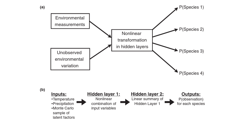
The last article I reported on examined stacked species distribution models (SDMs) to predict species richness across a landscape. This paper extends the idea of using SDMs for studies at the community level, incorporating information ignored by stacked SDMs (i.e., data on species co-occurrences). One method that incorporates data on species co-occurrences is joint species distribution modeling (JSDM). Here, the author extends this approach using a stochastic neural network approach (which he refers to as mistnet). This approach is compared to two common approaches. First, a stacked SDM of trained boosted regression models for each species. Second, a deterministic neural network approach. All approaches used breeding bird survey data. These data were split into train and test sets, where test data consisted of 280 routes and the training set of 1559 routes, separated by a 150 km buffer (see Figure 2 from paper). The deterministic neural net performed comparably to mistnet in predicting species occurrence probabilities, but mistnet outperformed the deterministic neural net when predicting community composition at a given site. The traditional joint SDM did not perform well in either task. The article doesn’t go into the tuning of mistnet (e.g., number of hidden layers), but it looks really cool, and all the code is available on Github.

A probabilistic approach to niche-based community models for spatial forecasts of assemblage properties and their uncertainties

Pellissier, Loïc, et al. “A probabilistic approach to niche‐based community models for spatial forecasts of assemblage properties and their uncertainties.” Journal of Biogeography 40.10 (2013): 1939-1946.


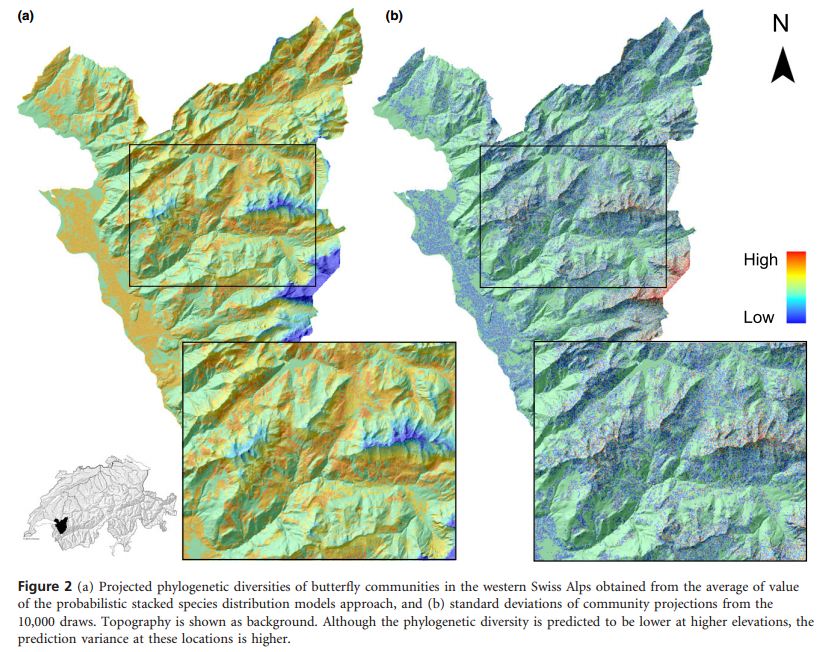
Species distribution models (SDMs) are typically developed for a single species, because most of the time the goal is to predict habitat suitability for the occurrence of a single species. However, could there be more information about latent environmental traits, or about the probability of species occurrence in data on the presences of other species? Probably. These authors investigated an approach to predict uncertainty in predictions of community properties from stacked species distribution models. Stacked species distribution models are simply a set of independently trained species distribution models that are then laid on top of one another to predict community composition or species richness across a landscape. They don’t incorporate co-occurrence data directly, which is a flaw in my opinion, and this is recognized and has been tackled in other papers. To assess the ability of stacked SDMs to predict species richness, the authors compared a hard threshold approach (each binary SDM was converted into presence-absence predictions, the sum of the predicted presences formed the species richness in a given cell), and a probabilistic approach (each SDM predicted a probability, and these probabilities were compared relative to a 10,000 draws from a binomial distribution). The latter approach resulted in a stronger correlation between expected and observed species richness values. Further, the authors argue that this approach gets at uncertainty in model predictions, by using the variability from the 10,000 draws to get at uncertainty. This demonstrates the utility in considering community context in species distribution modeling. Methods directly incorporating information on co-occurring species will likely provide an even better view of the realized niche of species, or of community composition across a landscape.

Grassland species loss resulting from reduced niche dimension

Harpole, W. Stanley, and David Tilman. “Grassland species loss resulting from reduced niche dimension.” Nature 446.7137 (2007): 791-793.


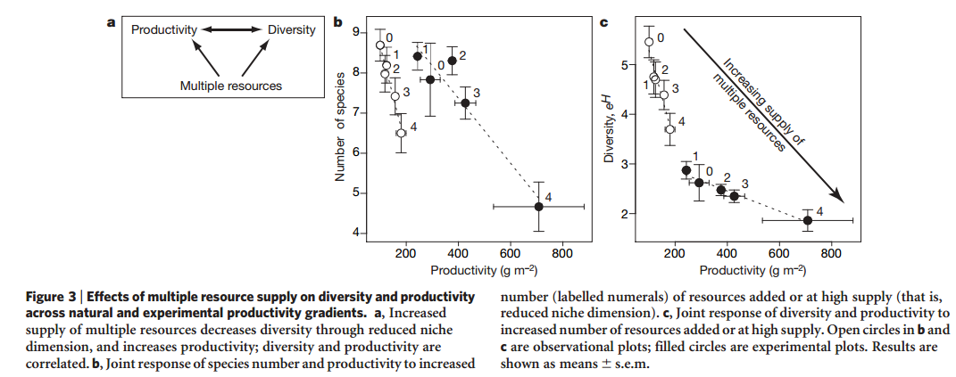
This study aimed to test a hypothesis derived from niche theory called the ‘niche dimension hypothesis’. This hypothesis posits that the addition of co-limiting resources should reduce species diversity while also increasing productivity. To test this, the authors used data on a previous enrichment study, combined with a similar experiment to get at the role of co-limiting nutrients on plant community dynamics in a grassland community. They varied the number of limiting resources they added (nitrogen, phosphorous, calcium, and water) in all possible pairs, finding that no one resource was strongly limiting, but many resources were co-limiting. They found the number of resources added was negatively and non-linearly related to the number of species in the community, but positively related to above-ground biomass. This suggests that a small subset of species are able to dominate in high resource environments, and is some of the motivating work behind the biodiversity-productivity navel-gazing fest that is currently taking place among ecosystem ecologists (see these papers).

I read this paper because I thought it was going to specifically discuss plant niches and dimensionality reduction. They use dimensionality to discuss the combined effects of the limiting nutrients on species diversity. They further argue for the possibility that competition isn’t the only factor in reducing species diversity, but that plants sensitive to nutrient additions could be exposed to abiotic conditions outside of their niche boundaries. They also discuss the effect of increased leaf litter, which is not a direct competitive interaction (like competition for light).

Model‐based uncertainty in species range prediction

Pearson, Richard G., Wilfried Thuiller, Miguel B. Araújo, Enrique Martinez‐Meyer, Lluís Brotons, Colin McClean, Lera Miles, Pedro Segurado, Terence P. Dawson, and David C. Lees.
Journal of Biogeography 33, no. 10 (2006): 1704-1711. doi:10.1111/j.1365-2699.2006.01460.x

This paper overall addresses the source of uncertainty in assessments of the impacts of climate change on biodiversity. Pearson et al. used a variety of environmental niche modelling techniques (artificial neural network, climate envelope range, constrained Gower metric, classification tree analysis, genetic algorithm, generalized additive model, genetic algorithm for rule-set prediction, and generalized linear model) to evaluate the impact (magnitude of variation) of model choice on predicted species distribution under current and predicted climate change scenarios and why model outputs may differ. They used data on four endemic plant species of Protoeacea found in S. Africa collected from 3996 sampled sites located within different 1’X1’ cells and used identical input variables that are considered critical to plant physiology and survival. Model predictions were compared by testing agreement between observed and simulated distributions for present day (using AUC and kappa statistics) and assessed consistency in prediction of range size changes under future climate using cluster analysis. Distribution was characterized by the number of grid cells occupied. Technique was applied to 70% randomly selected sites and 30% was used to test agreement between observed and modelled distributions. Under climate change scenarios, for all models, except CER and GA, the suitability for each cell was calculated at decision thresholds increasing from 0-1 and used cluster analysis to group predicted ranges from different methods under current and future climate conditions. They found that: variation between model predictions can be attributed to models that use presence-only data vs. presence-absence data (so realized vs. fundamental niche predictions) as they had performed differently. Another key factor that should be carefully considered for ENMs is model extrapolation assumptions. For example, instances of extrapolating environmental variables under climate change range expansion yielded uncertainty in model predictions. Similar to class discussion this week, this paper presents models on an endemic (and plant) species, it would be interesting to apply the same objective to a non-endemic vertebrate species and compare model predictions.

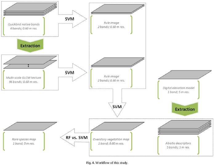
Support vector machines to map rare and endangered native plants in Pacific islands forests

Pouteau, Robin, et al. “Support vector machines to map rare and endangered native plants in Pacific islands forests.” Ecological Informatics 9 (2012): 37-46.
doi:10.1016/j.ecoinf.2012.03.003

Occurrence records are scarce for rare species, which results in small training sample available for species distribution models. Support Vector Machine (SVM) was traditionally used in remotely sensed data classification for classifying object reflectance, which is substantially the same than classifiers used in species distribution models. Since the decision made by SVM is solely based on few meaningful pixels, this method is much appropriate for predicting distribution of species with scarce occurrence records. Pouteau et. al. compared two machine-learning methods, random forest (RF) and SVM, to determine which method is the most relevant to map rare species and to predict potential habitat with their current observed range. The comparison was performed using three rare plants found at the island of Moorea. Biophysical variables including elevation, climate, geology, soil substrate, disturbance regime, floristic region, plant dispersal capacities, and ecological plant type and function. Their results showed that SVM preformed constantly better than RF in distribution prediction in terms of Kappa coefficient and the area under the curve (AUC). In this case, the predicted distribution generated from SVM has high enough accuracy with only 13 training pixels. This was contributed by the ability of SVM to train model with few meaningful pixels and fit limitation information and the ability to resist noise from insignificant pixels. By comparing species potential habitat with current observed range, we will be able to better understand the causes of the conservation status of the targeted species. So far, there are only limited applications of SVM for special distribution models. It would be interesting to repeat the application for other rare plants or animals.

Capture

Evaluating predictive models of species’ distributions: criteria for selecting optimal models

Anderson, Robert P., Daniel Lew, and A. Townsend Peterson. “Evaluating predictive models of species’ distributions: criteria for selecting optimal models.Ecological modelling 162.3 (2003): 211-232.

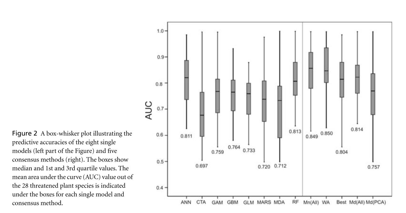
Anderson et al. assess the utility of consensus based predictors in species distribution models. These consensus predictors are made up of a number of fitted species distribution models of varying types. Component SDMs used for consensus modeling were GLM, GAM, MARS, ANN, GBM, RF, CTA, and MDA. These individual models were trained and evaluated on appropriate sub-subsets of the 70% training data subset in order to pre-evaluate these models for the purpose of consensus modeling. Consensus models assessed include Median(All) and Mean(All) which use the median and mean, respectively, of the predictions of all 8 models. The WA approach determines the 4 models with highest accuracy for a given species and computes a weighted average of their outputs. Median(PCA) is calculated as the median of the 4 models for which the variance of the predictions along the 1st principle component of a PCA was the greatest. Finally, Best simply selects the best individual model based on the highest pre-evaluated AUC value. Each of these methods, as well of each of the individual models, were then evaluated using the 30% testing data subset. WA and Mean(All) provided significantly more robust predictions than all single models and all other consensus methods. WA was the best model with a mean AUC of .850 and better predictive performance than all single-models on 21 of 28 species. These methods provide a functional alternative to thorough single-model evaluation and comparison. The fact that the true consensus models consistently outperform the “Best” consensus model suggests the utility of these methods over comparative evaluation. These consensus models also effectively address the common issues that some single-models provide better predictions for interpolation and some for extrapolation and that the best evaluated model often varies significantly from species to species.


Anderson figure