Are richness patterns of common and rare species equally well explained by environmental variables?

Lennon, J. J., et al. (2011). “Are richness patterns of common and rare species equally well explained by environmental variables?” Ecography 34(4): 529-539.

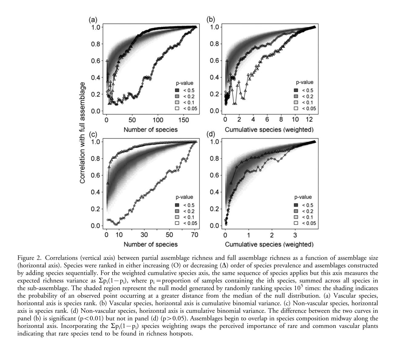
Species richness predictions based on environmental models rely on the assumption that richness patterns of both common and rare species respond similarly to environmental variables. Additionally the contribution of rare species to variation in richness may be swamped out by the contributions of more common species meaning that environmental factors identified as important for richness may just be important for this small subset of influential species. This phenomenon may be driven by the skewed distribution of species commonness, namely that rare species are rarer than common species are common. So in a small assemblage of rare species there will be many areas with 0 richness, while a similar size assemblage of common species will have fewer areas of uniform richness (fewer 0s but still not many maximums). This paper focuses on showing how species along the rare-common continuum differ in environmental associations using grassland plant and lichen species along an environmental gradient on the Scottish island of South Uist. Hypothesis: Rare species associated with rare environments and common species with common environments and rare and common species differ in relation to environmental variable. 217 roughly evenly spaced samples were taken along a 200mX2162m grid. At each site species composition along with soil and environmental variables were recorded. To determine the effect of rarity on contribution to richness sub-assemblages were built sequentially from most common and least common species, correlated richness values for each individual sub-assemblage with the total assemblage and plotted them against rank order of species addition. In order to account for the relative capacity of species to contribute on the basis of their prevalence alone correlations were also plotted against the expected variance of the given sub-assemblage richness pattern. These correlation plots were compared to an iterated null model. Common species contribute more to species richness patterns than rare species. When expected variance due to prevalence is taken into account this pattern reverses for vascular plants with rare species more associated with higher richnesses. The rescaling of non-vascular plants that there may not be a clear relationship between rarity and richness. GLMMs with Poisson errors and exponentially spatially structured random affects fitted using penalized quasi-likelihood were fit to each pattern of building species assemblages, with species richness as response. Small assemblages of rare species are poorly explained by environmental covariates as compared to common species. For vascular plants richness vs. environment associations of common species differ from those for rare species. For non-vascular plants models fit to more common species fit better likely due to them being easier to predict. Similar GLMMs were fit to the relationship between the species richness of each assemblage along the rare-common axis as a function of the environmental rarity and extremity of the sample (in environmental space). For vascular plants, rarer species were significantly positively associated with extreme and rare environments while commoner species were associated with only moderate environments. For non-vascular plants, only common species were associated with moderate and rare conditions. This is despite the fact that environmental rarity and extremity are strongly correlated (r=0.84). Clearly common and rare species can both respond differently to environmental variables and differentially affect species richness while the responses differ between vascular and non-vascular plants.
 

beale figure

Spatial autocorrelation in predictors reduces the impact of positional uncertainty in occurrence data on species distribution modeling

Naimi, Babak, et al. “Spatial autocorrelation in predictors reduces the impact of positional uncertainty in occurrence data on species distribution modelling.” Journal of Biogeography 38.8 (2011): 1497-1509.

Link

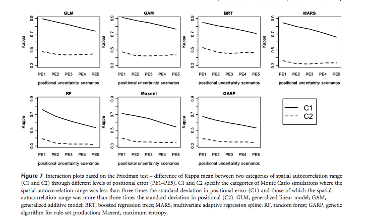
This study investigates how using information regarding spatial autocorrelation of environmental variables can help mitigate the error introduced from positional uncertainty in species occurrence data. Spatial autocorrelation refers to the idea that for any given point in space of an environmental variable one would expect the nearby surrounding points to be more similar compared to those that are further away. Position uncertainty results from errors in determining where the geographical occurrence of the observation took place. In this study researchers used a simulated data set to observe how the interactions between spatially autocorrelated variables and positional error can influence the predictions made in both presence-only and presence-absence SDMs.

Screenshot 2016-05-01 13.54.41

The simulated artificial data set was comprised of 2 environmental variables and one set of species observations that was linked to the environmental gradient. Researchers incorporated errors into their observation data based on a normal distribution, and then further propagated the uncertainty with Monte Carlo simulations. Species distribution models were evaluated using AUC and Cohen’s Kappa statistics. Cohen’s Kappa is a proportional measure that is variable to the set threshold detection level (unlike AUC). A two-way Friedman’s test was employed to asses if SAC in predictors reduced the influence of positional uncertainty.
Results showed that model performance varied depending on the trade between the degree of positional uncertainty and spatial autocorrelation in the provided data set. It is possible for spatial autocorrelation to reduce the impact of positional error; however, it is unable to fully compensate for error when positional error is extreme. Boosted regression trees, Generalized additive models, and Generalized linear models all outperformed random forests, Garp, and Maxent in terms of AUC. This is explained by the fact that the better performing models are presence-absence and thus have more information to make their predictions on.

Species distribution models and ecological suitability analysis of potential tick vectors of Lyme Disease in Mexico

Lyme disease, a a tick-borne disease caused by Borrelia burgdorferi,  has had an increasing number of cases occur in Mexico.  While the disease is rare in the Southern United States, it has been found to occur in Northern and Mid-Western US and Europe.  The authors investigate the distribution of potential tick vectors (ten Ixodoes spp. and Amblyomma cajennense [inclusion of this species as a vector is through personal communication]) in Mexico.

Occurrence data of the ticks was collected from prior publications and field surveys.  However, the occurrence data for ticks in Texas and Mexico was too sparse to do the models independently.  While the data used was collected in both Mexico and Texas, the authors only present the results for Mexico.  Environmental data was collected from WorldClim.  The distribution model used was MaxEnt and the trained for the Amblyomma cajennense  and the ten Ixodoes as a group.

JTM2012-959101.003

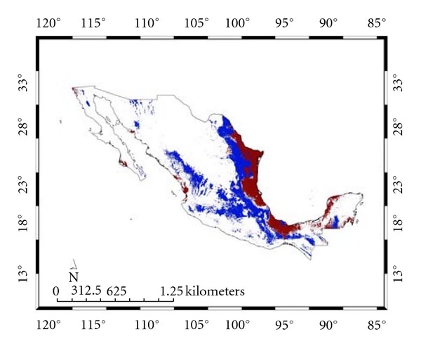
From the results, there is spatial non concordance between the species.  Amblyomma cajennense  was mainly predicted to occur in mangrove and marsh regions at lower altitudes along the coast (red region).  The Ixodoes group are mainly found in oak and pine-oak forests.  These results highlight that if a species in the Ixodoes group is capable of transmitting the pathogen then the areas of highest risk are at high-altitude low temperature areas (which helps explain why Lyme disease is so rare in the southern US, high temperatures). However, if it is true that Amblyomma cajennense is capable of maintaining the pathogen in reservoir hosts, then the region extends  eastern lowlands of Mexico.

Illoldi-Rangel, P. et al. 2012 Species distribution models and ecological suitability analysis for potential tick vectors of Lyme disease in Mexico. J. Trop. Med. 2012.

Comparative interpretation of count, presence-absence, and point methods for species distribution models

Link

This study compared the likelihood functions used in species distribution modeling that have differences in occurrence records such as presence-only, presence-background, and presence-absence. Specifically, researchers focus on the differences of point and count data. Results indicate that the differences between the likelihood function of count data, and the likelihood function for point methods can originate from the same underlying inhomogeneous Poisson point processes model.

To first accomplish this, researchers provide an equation that allows for the consideration of continuous environmental space instead of discrete environmental space (equation 1). Researchers then adapt geographic space from discrete to continuous. They then provide considerations for the response type given either a discrete or continuous environmental/geographic space. After addressing these points, researchers then present the likelihood functions for unconditional inhomogenous Poissoin point processes and conditional inhomogenous Poisson point processes, and indicate how both functions are related to the Poisson log-likelihood.  

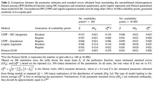
To asses how parameter estimates might vary across different realizations of the species range, researchers conducted a simulation and compared differences between IPP and logistic regression using either 100 or 10,000 availability points and one spatially autocorrelated environmental variable. To generate different parameter estimates the creation of environment and occurrence observation was repeated roughly 500 times. The mean estimates were compared to the true values; as well as, using Monte Carlo standard deviations. Most models were able to capture the true parameter value; however, the Poisson GLM performed poorly compared to all other models. The reason provided is because the scale the environmental covariate was distributed was much smaller than the resolution of the grid cells.

Screenshot 2016-05-01 10.38.04


Applications and future challenges in marine species distribution modeling

Dambach, Johannes, and Dennis Rödder. “Applications and future challenges in marine species distribution modeling.” Aquatic Conservation: Marine and Freshwater Ecosystems 21.1 (2011): 92-100.

Link

This study highlights how the effects of climate change are altering marine species distributions and also highlights challenges unique to marine species distribution modeling. Researchers posit that increasing ocean temperatures will force species to shift either in latitude or depth with accompanied tradeoffs with respect to the selected shift. As a consequence invasions and local/global extinctions are expected to continue to increase.

Authors provide three points highlighting unique challenges within marine species distribution modeling. First, authors consider how complex three dimensional structure generates the need to understand how depth influences contributing factors. Related to the three dimensional complexity issues is that preference in depth can differ depending on the life stage of the species in question (eg: larval and adult stages). One possible solution is to apply species distribution models at varying stages of depth, then layer predictions appropriately. Second, dispersal via ocean currents is a significant driver of many marine in some instances more important than local physical properties themselves. Lastly, there exists a known bias in occurrence records between coastal and open water surveys. Which can complicate knowledge of habitat preference for species that occupy both at some point in their life cycles.

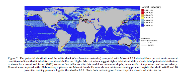
This paper also presents a case study on great white sharks, Carcharodon carcharias, habitat suitability. The great white shark is a suitable organism to model due to its known global migration patterns. White shark occurrence records were accessed through GBIF. Environmental parameters considered were the following: minimum depth, sea-surface temperature, and salinity. Researchers used MaxEnt and a Last Glacial Maximum output to determine how white shark distribution could change under climate change. Outputs suggest that white sharks are more likely to adjust their distributions to increased latitudes in the future due to changes in environmental conditions. Given that the white shark is an apex predator this could further create consequences for other animals currently occupying the predicted expansion areas.

Screenshot 2016-05-01 10.35.55

How many predictors in species distribution models at the landscape scale? Land use versus LiDAR-derived canopy height

Ficetola, Gentile Francesco, et al. “How many predictors in species distribution models at the landscape scale? Land use versus LiDAR-derived canopy height.” International Journal of Geographical Information Science28.8 (2014): 1723-1739.
Link

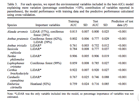
In this study researchers employ an approach to better evaluate which features of the landscape, mainly those measured by remotely sensed tools, are important for a selected bird sanctuary in the Netherlands. They define their study as being small with no variability in climatic or topographic gradients, which provides reason to suggest that features of the landscape are driving species distribution. Using data collected from a Biodiviersity Multi-SOurce Monitoring System: From Space to Speices (BIO_SOS) project, researchers compared the performance of five different models in explaining species distribution provided a fine scale study area.


Models

  1. Models using a relatively large number of traditional land-use variables
  2. Models using a small number of land-use variables
  3. Models excluding land-use variables, and only using canopy height collected via LiDAR sensors
  4. Models using a large number of land-use variables and LiDAR
  5. Models using a small number of land-use variables and LiDAR


Occurrence data was collected within the Veluwe located in the Netherlands, the Veluwe is roughly equivalent to a national park found within the United States. Land-use/land-cover data sets were collected through the Dutch government, and the likely satellite system used to collect the base images were Landsat. Seven classified habitats were included in this study: broadleaved forest, coniferous forest, heathland, grassland, sparse vegetation, built-up, and shifting sand. The study area was partitioned into 20 m x 20 m cells, and for each cell researchers measured the average cover of habitat within a 100 m radius from the cell center. LiDAR data was also attributed to cells in the same way.

For Analysis, researchers first determined the correlation coefficients between independent variables with |r| >0.7 as a cut off. They also used a variance inflator factor to determine whether multicollinearity occurs in developed models. MaxENT models were built for predicting species distribution.

Results indicated that in general there was a lack of collinearity between environmental variables (|r| < 0.7), with the exception of canopy height being positively related to coniferous forests and negative to heathland and a negative relationship between forest and heathland. Seven out of the nine species of birds evaluated using MaxENT were found to be best predicted using LiDAR provided information with the majority of models performing best with LiDAR only information. This finding suggest that increased detail in provided environmental information (eg: LiDAR) will provide, in general, better fit models for predicting species distributions. Provided the measured environmental information is relevant to predicting the occurrence of the focal species.

Screenshot 2016-05-01 10.32.36

Geographic distribution of Chagas disease vectors in Brazil based on ecological niche modeling

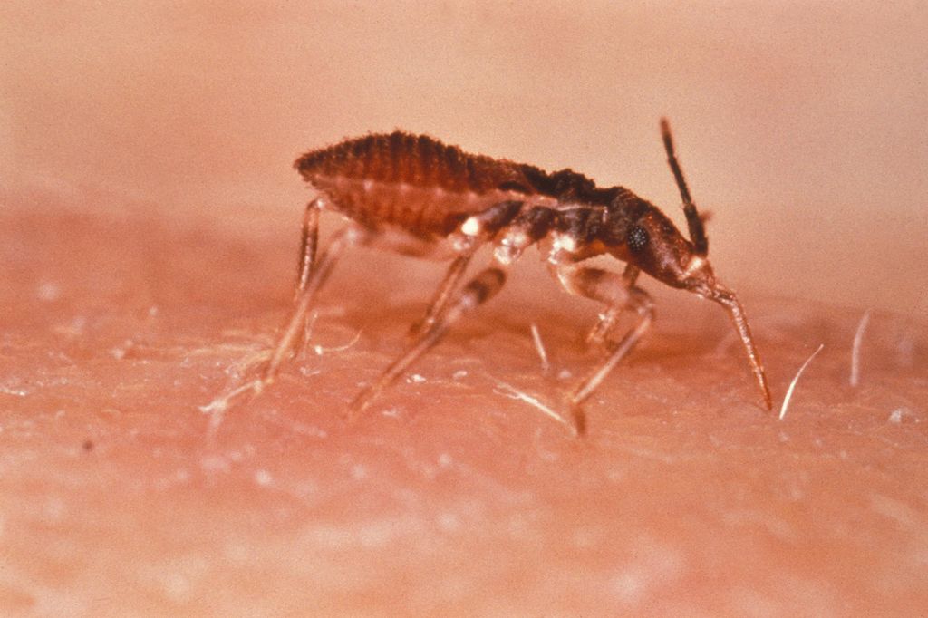
Chugs disease is caused by Trypanosome cruzi parasite which is primarily transmitted through kissing bugs (triatomines).  While control measures have been implemented to help control the domestic vector population in Brazil and have shown to be effective in reducing disease occurrence, there are still reported cases of the disease transmitted from the native vectors. These occurrences can be there result of sylvatic vectors invading households, contamination of food, or domestic/peridomestic vectors.  The authors investigate the distribution of 62 Brazilian species of the vectors.

MaxEnt was used to model the distributions.  Occurrence data for the species was collected from multiple sources including Brazilian State Health Departments. Environmental data was used from two datasets: multitemporal remotely sensed imagery (Advanced Very High Resolution Radiometer satellite) and climatic variables (WorldClim). Of the species modeled, P. geniculatus and P. megistus had the largest/broadest distribution.

705326.fig.008

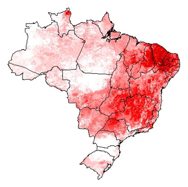
Species diversity map, darker red regions have higher predicted cooccurring species.

The most favored regions for the vectors are the Cerrado and Caatinga, the diagonal open areas in eastern South America.  The results also highlight the nowhere in Brazil is Chagas risk small but some regions are of higher risk than others. Also, the current distribution of T. infestans (the domestic vector) shows the impact and effectiveness of the control measures.

Gurgel-Gonçalves, R., Galvao, C., Costa, J. & Peterson, A. T. 2012 Geographic distribution of Chagas disease vectors in Brazil based on ecological niche modeling. J. Trop. Med. 2012.

Predictive distribution modeling with enhanced remote sensing and multiple validation techniques to support mountain bongo antelope recovery

Estes, L. D., et al. “Predictive distribution modeling with enhanced remote sensing and multiple validation techniques to support mountain bongo antelope recovery.” Animal Conservation 14.5 (2011): 521-532.

DOI: 10.1111/j.1469-1795.2011.0045

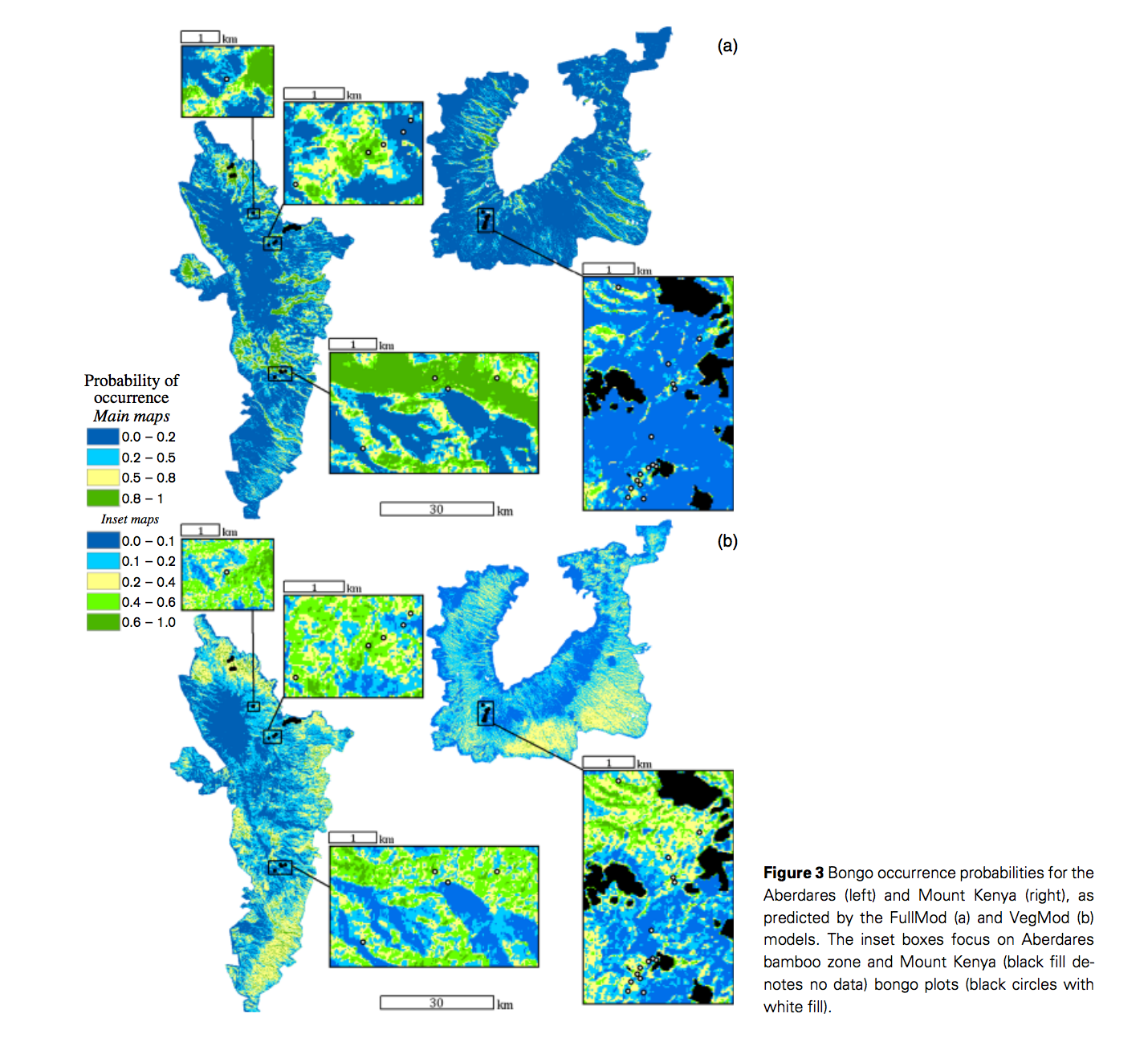
Transferable predictive distribution model is based on predictors describing the ranges and scales of relevant environmental gradients It is able to predict distributions of habitat use so that to facilitate species recovery. Estes et al used logistic regression modeling approach for a rare species, mountain bongo, to understand their special ecology of habitat use and to assist species recovery in Mont Kenya and Aberdares. One common problem for species distribution modeling for rare species is data limitation. They used remote sensing derived quantitative vegetation structure maps, moisture, and ruggedness as transferable habitat predictors. Totally 31 logistic linear regression models were constructed and tested using AIC values. A DNA analysis was applied to verify observations of bongo. They also used independent observations from Mont Kenya to assess the transferability of the model. The models showed ruggedness was the most important variables for habitat use, indicating their strong preference to difficult terrain. Bongos also prefer sites that closer to the patrol route of park rangers and that have complex vegetation structures. However, predictors are sources of model bias when transfer models between habitats, such as over-parameterization and spatio-temporal variation in species-environment relationships. Estes et al stated that bongo habitat associations should not differ greatly between two habitats, but the environmental variations between mountains caused the limited transferability of the mountain. As predictors, elevation is indirect as oppose to vegetation and moisture, which are directly related to habitat use. A direct measures of predation risk and food plant abundance and using better-sourced remote sensing imagery would improve this model, which is highly dependent on remote sensed data.

Screen Shot 2016-05-01 at 8.58.15 AM

Mapping large-scale bird distributions using occupancy models and citizen data with spatially biased sampling effort

Higa, M., et al. (2015). “Mapping large-scale bird distributions using occupancy models and citizen data with spatially biased sampling effort.” Diversity and Distributions 21(1): 46-54.

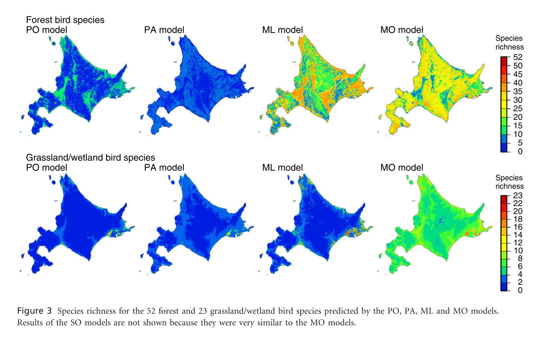
Citizen science data offers the ability to collect large amounts of species distribution data that would be impossible for a researcher to gather otherwise. This data can, however, suffer from issues of inconsistent data quality across the range (because of inconsistency in the expertise of citizens) and spatial sampling bias. The authors consider multiple SDM methods and their performance when applied to an aggregated data set collected by professionals and citizens with spatially biased sampling effort. Records of bird species presences were sorted into 4 categories: point census by experts, line census by experts, observation with other methods by experts, and observation with other methods by citizens. Environmental covariates were land cover and elevation. Models employed were presence-absence (PA) or presence-pseudoabsence (PO) (depending on available data) logistic regression, MaxLike, and two types of occupancy models. One type of occupancy model analyzed each species individually (SO) while another analyzed multiple species in the same model (MO). Both of these models depend estimation of latent occupancy (a Bernoulli variable) and detection/non-detection (a Bernoulli variable based on occupancy and observation probability from detection/non-detection data. The SO models for 18 forest bird species and two grassland/wetland bird species did not converge. Detection probabilities for all species were below 1 and differed by observation type (line census by experts>other methods by citizens and point census by experts>other methods by experts). Probability of presence for forest species decreased with forest area for PO and ML models while it increased with forest area in PA and especially occupancy models. Grassland/wetland species probability of presence increased with grassland and/or wetland area across all models though species richnesses predicted by PA, PO, and ML were lower than occupancy models. Both types of occupancy models (SO and MO) generally agreed. The authors claim that this work demonstrates the weakness of MaxLike and presence-only logistic regression in the face of spatial sampling bias. They put forward occupancy models that explicitly model detection as an easier and equally effective method as, if not a more effective method than, accounting for bias through similarly biased absence data (PA). Though this study lacks any actual evaluative measures (beyond the assumption that forest species should be more likely to occur in larger forests), the process of occupancy modeling seems nonetheless very promising and should certainly be tested more broadly.


higa figure

Model-Based Control of Observer Bias for Presence-Only Data in Ecology

Warton, D. I., et al. (2013). “Model-based control of observer bias for the analysis of presence-only data in ecology.” PLoS One 8(11): e79168.

Observer bias can be a major problem in building SDMs with presence-only data. The authors define observer bias as the idea that “a species is more likely to have been recorded as occurring in a place where people are more likely to see and record it.” Using presences for other sampled species as pseudo-absences for your model is one way of addressing this issue if we assume that observer bias is consistent across species. The paper considers two alternative ways of implementing this approach: a point based approach and a grid cell based approach (in which records within a grid cell are aggregated such that a presence point in a grid cell means that that cell is a presence record for the focal species or the non-focal species respectively). This approach may replace observer bias with species richness bias, by restructuring our question to one of species composition. We now ask, given we at least one species is present in a cell/point, what is the probability that it is our focal species. The authors, therefore, propose an alternative, model-based bias correction method which they compare with these earlier methods. This method consists of modeling the likelihood of observing a presence as a function of both environmental variables and “observer bias variables” such as accessibility of sites. These functions are assumed to be additive. In order to control for observer bias during prediction all observer bias variables are set to a constant across all prediction points/cells. All analyses are performed using a Poisson point process regression model with a LASSO penalty for variable selection. First the authors work through an illustrative example with a single species Eucalyptus apiculata. The model fit with environmental variables and the model fit with environmental and observer bias variables are relatively similar with the second providing a better fit to presence points. The model fit to both types of variables and then controlled for observer bias provides a very different distribution with positive predictions extending into low accessibility areas. In order to draw broader conclusions they trained and evaluated models using 5-fold cross-validation on a presence-absence data set containing 62 species. 84% of species were better predicted when using model-based bias correction than when ignoring bias. These improvements were on average relatively small (95% CI for increase in AUC: 1.5+/- 1.1). Significantly more species were predicted better by model-based bias correction than by the alternative pseudoabsence approach described above. Some species were, however, fit better by the pseudoabsence approach. Potential pitfalls of this new model-based bias correction approach include: a reliance on the quality of the variables chosen to quantify observer bias and on the ability for the effect of these variables to be estimated from the available presence records (making small numbers of records particularly problematic), and the reduction in effectiveness that will come from (likely quite common) correlations between environmental and observer bias variables. This method seems relatively effective and very well grounded conceptually. It would be interesting to see it compared to other common methods of bias reduction beyond the pseudoabsence approach.