The role of biotic interactions in shaping distributions and realized assemblages of species: implications for species distribution modeling

As with Mod (2015), the integration of biotic interactions/variables into species distribution models is of interest.  It is already know that at small, local scales biotic interactions influence the distribution of species.  However, in order to integrate these interactions at a larger scale and in the future, a better understanding of how these interactions have influenced the species historically and dispersal.  The authors provide a review using studies involving species ranges, functional groups, and patterns of species richness.

The authors find that the biotic interactions have shaped the distribution of species beyond the local extent (10 km^2). The authors then suggest and review some ways to integrate biotic interactions within species distribution models.  These include using pairwise dependencies, using integrative predictors, and lastly hybridizing the models with dynamic models.

However, there are some problems with integrating these.  One possible problem is that species interactions may not be constant in time and space.  All the integrated models would assume that the interaction would be static between species. Any changes in species composition may affect these interactions through time and also space.  The authors close by calling for better data collection across scales and along environmental gradients.

Wisz, M. S. et al. 2013 The role of biotic interactions in shaping distributions and realised assemblages of species: implications for species distribution modelling. Biol. Rev. 88, 15–30.

Using species distribution modeling to delineate the botanical richness patterns and phytogeographical regions of China

Due to the recent archiving and georeferencing of plant specimen collected over the past century, the distribution modeling of these species is now easily possible. The authors modeled the distribution of 6,828 species and determined the biological richness of areas in China.  In addition, they also investigated the drivers of the richness in the areas.

To prediction the distribution of the species, they used MaxEnt.  To analyze regions of species richness, they used ordination and Getis-Ord Gi* statistics finding hotspots of species richness. These also allowed them to determine the drivers of species richness and hotspots.

srep22400-f1


Of the predictors used, annual precipitation and temperature stability provided a major role in the observed species diversity.  However, when looking at the different regions, there were different drivers:

  • SE – annual precipitation
  • SW – topographic & temperature stability
  • NW – water deficit
  • NE – temperature instability


srep22400-f3

Fifteen uncorrelated variables plotted as predictors of environmental turnover calculated for 6560 woody species. Vectors are displayed only for the highly significant variables (P < 0.001) inferred from non-metric multidimensional scaling (NMDS) ordination. TAR: Temperature Annual Rang.

Zhang, M.-G., Slik, J. W. F. & Ma, K.-P. 2016 Using species distribution modeling to delineate the botanical richness patterns and phytogeographical regions of China. Sci. Rep. 6.

Modeling hotspots of the two dominant Rift Valley fever vectors (Aedes vegans and Culex poicilipes) in Barkédji, Sénégal

In relation to Mosomtai et al. (2016) (see Association of ecological factors with Rift Valley fever occurrence and mapping of risk zones in Kenya) these authors predict the distribution of the two vectors for Rift Valley fever (RVF).  Previous studies have looked at disease risk by finding areas with high vectors pressure or virus activity.  Here the authors investigate the impact of climate and environment on the presence of Aedes vegans and Culex poicilipes  (the two primary vectors of RFV).

13071_2016_1399_Fig1_HTML

Mosquito data was gathered from the Barkedji village (Ferlo area) during 2005 to 2006 across 79 sites.  After collecting the data, the Getis-Ord statistic was calculated to determine hotspots (adult mosquito abundance clusters).  The Getis-Ord Gi* measures the spatial clustering by identifying hotspots with a higher magnitude than expected from random chance. To deal with spatial autocorrelation, generalized linear mixed effect models were used.  The response/dependent variable was the calculated Getis-Ord Gi* of the hotspots.  The predictor/independent variables were rainfall, relative humidity, max and min temperature, NDVI, and distance from nearest pond.

13071_2016_1399_Fig6_HTML

For the Culex species, drops in the minimum temperature allows for an increase the occurrence of hotspots.  For the Aedes species, there is a negative relationship with relative humidity, max and min temperatures and hotspot occurrence. For both species, the distance to the nearest pond increases the occurrence of a hotspot. The authors close the paper by commenting that these models and understanding what promotes the occurrence of hotspots can lead to better vector control in the area.

Talla, C., Diallo, D., Dia, I., Ba, Y., Ndione, J.-A., Morse, A. P., Diop, A. & Diallo, M. 2016 Modelling hotspots of the two dominant Rift Valley fever vectors (Aedes vexans and Culex poicilipes) in Barkédji, Sénégal. Parasit. Vectors 9, 1.

Estimating species diversity and distribution in the era of Big Data: to what extent can we trust public databases?

Maldonado, C., et al. (2015). “Estimating species diversity and distribution in the era of Big Data: to what extent can we trust public databases?Global Ecology and Biogeography 24(8): 973-984.

The vast records of species distributions contained in natural history collections are rapidly getting digitized and becoming widely available online. These data provide an invaluable resource for Species Distribution Modeling. One of the largest biodiversity databases is the Global Biodiversity Information Facility (GBIF). Despite increasing quality of data researchers should retain a critical eye for poor quality of geographic positions or erroneous taxonomic identifications. The researchers ask to what extent data in the GBIF are sufficient for prediction of distribution patterns using data for the plant tribe Cinchoneae in the Neotropics. Three data sets were taken from GBIF: (1) a non-cleaned dataset (3720 records), (2) a cleaned dataset (3572 records), (3) and a cleaned dataset with the manual addition of records from other sources (3756 records). A fourth dataset (VD) was compiled manually through classical taxonomic work using the main herbaria in South America and the Missouri Botanical Garden (2670 records). Species distribution and species richness were analyzed on all four datasets at three spatial scales using SpeciesGeoCoder. Scales are grids (one-degree cells covering the entire range of the tribe), Ecoregions (defined by WWF), Biomes (polygons also defined by WWF). Distribution and richness were also analyzed by altitude. At the grid scale the basic GBIF data identified a number of richness hotspots not identified by VD these were noted to be a result of records with country level locality data which was converted to point data using the center of the country. These erroneous hotspots were not present after data cleaning because these rough locality measures were those preferentially cleaned. At the ecoregion level, in general, ecoregions in the central areas of a number of countries had higher richness under GBIF records than VD records as a result of the poor georeferencing described above. The number of species per ecoregion was not, however, consistently higher for GBIF. At the biome level the main discrepancy is a much larger number of species in the “Tropical and Subtropical Grasslands and Savannas and Shrublands” biome under VD (34) records than GBIF (10), again a result of georeferencing errors. As above the GBIF cleaned and GBIF cleaned and increased data sets more closely approximated VD. Increasing spatial scale did not ameliorate the effect of these errors. In contrast GBIF and VD widely concur in the altitudinal ranges of species.

GBIF records have the advantage of more participating institutions and consequently more records cheaply and in a uniform format but are still plagued by taxonomic and, most notably for this analysis, georeferencing errors. Data cleaning seems to deal with some forms of georeferencing errors relatively effectively. The authors also suggest raising minimum requirements for data submission and peer-review of data in order to increase GBIF data quality before the end user.


maldonado figure

Bias correction in species distribution models: pooling survey and collection data for multiple species

Fithian, W., Elith, J., Hastie, T., Keith, D. A. (2015), Bias correction in species distribution models: pooling survey and collection data for multiple species. Methods in Ecology and Evolution, 6: 424–438. doi: 10.1111/2041-210X.12242


Presence only records are common for rare species, but are often biased due to a haphazard collection schemes. The authors propose a correction for this bias by using presence – absence data with similar geographic sampling biases from other species.

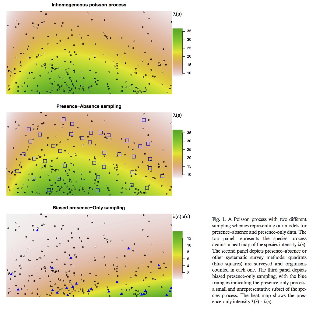
Most popular presence only models are motivated by an inhomogeneous Poisson process (IPP). The IPP for a single species presence only data can be extended to adjust for sampling bias by incorporating presence – absence data from multiple species into a single joint probabilistic model to estimate and adjust for bias. The authors evaluate their model using both presence – only an presence – absence data for a set of Eucalypt species from south–eastern Australia (R package multi–speciesPP). Presence – only point processes can be thought of as a thinned presence – absence point process. How and where the thinning occurs is biased by opportunistic presence only sampling. See figure 1 for visual explanation. This means, at best, presence only IPP estimate relative intensities not probabilities of occurrence. This is due to the identifiability issue of parameters in the thinned intensity function.

wk10_Fig1

Previous attempts to correct for this bias have included factors that lead to sampling bias such as distance from roads and population centers. However, these corrections only work if they do not correlate with environmental variables. In Australia large populations are clustered along the East Coast, but important climatic variables are also correlated with distance from the same coast.

The authors propose using a joint log linear IPP model for multi-species data, a subset of which are presence – absence data. The point process and send point process are both assumed to be independent across species with a log linear intensity and bias, however bias intercept (delta) is not allowed to vary across species. This restriction assumes that bias is proportional across species which allows the authors to pool the information into a single estimate – deriving the bias of presence only data from presence absence data.

Testing the method:

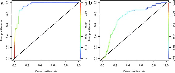
The Eucalypt data set consists of 36 species at 32,612 sites with an average of 547 presences per species. However, this range is variable 4 species have fewer than 20 observations and 8 having more than 1000. The presence only data consists of 764 observations supplemented with 40,000 background points. The authors evaluated their methods by assessing the assumption of proportional sampling bias, and the impact of pooling multiple species on predictions.

The proportional bias assumption was found to be appropriate in some species, and inappropriate in others. Pooled data had the greatest impact on model performance when the presence absence data for species of particular interest were either scarce or nonexistent. The authors  acknowledge the proposed method has many shortcomings, but point out that it performs better than models with no sampling bias correction.

Delimiting the geographical background in species distribution modelling

Acevedo, P., et al. (2012). “Delimiting the geographical background in species distribution modelling.Journal of Biogeography 39(8): 1383-1390.

The role of the geographical background (GB) extent is clearly an important one in the field of Species Distribution Models. Notably an increased extent of GB can artificially inflate the perceived discriminatory power of an SDM by adding many uninhabited and unsuitable sites. And if unoccupied but environmentally suitable areas are used for model training then predictive capacity may be reduced. As an alternative to the methods of Barve et al. (2011) the authors propose trend surface analysis (TSA) as a way to determine the GB that maximizes the likelihood that the targeted species is interacting with the environment (i.e. areas that are otherwise accessible). The trial analysis was performed on four native ungulate species in mainland Spain. A third degree TSA was fitted (for processes that occur at the same or a higher spatial scale than the study area) the basic GB (GBLOW) was delimited by selecting all points with the lowest TSA value assigned to a presence or greater. Then the GB was restricted by excluding 1%, 5% and 10% of the presences with the lowest TSA values and extended by including 1%, 5%, and 10% of the absences with the highest TSA values, lower than the value of any presence. Logistic regression models were trained on a 70% random sample fo the data. Predictive performance was assessed on three evaluation data sets: (1) the remaining 30% of the training data within the GB, (2) only evalutation data in GB-10%, (3) using all the localities in GB-10% for all species. TSA results showed broad-scale spatial trends in species distributions. Predictions of all models are quite similar in the core area and highest variability between different models is found when making predictions outside the training data sets. There was a negative association between AUC and GB extent when assessed on core areas and a positive association when evaluated on the training area. There was also a negative association between GB extent and the area of Spain predicted as suitable. Increasing GB produces models that appear better (higher AUC) but that are barely informative. Larger areas of suitability predicted by smaller GBs were also more in accordance with expert opinions. This TSA approach seems to offer a more easily implemented alternative to Barve et al. (2011) for estimating the parts of the landscape to be designated as ‘M’ or the accessible area and could perhaps be used effectively in a broad array of contexts.

avecedo figure

Ten Simple Rules for Reproducible Computational Research

Sandve, Geir Kjetil, et al. “Ten simple rules for reproducible computational research.” PLoS Comput Biol 9.10 (2013): e1003285.

Link

Scientific research has seen a rise in recent years of the increasing demands for more computational skills required to conduct biological and ecological research. This increase in research complexity has precipitated the need to stress the importance of reproducibility of computational methods. Reproducibility is an abstract concept that provides a way to consider how likely someone else provided your data and methods could recreate the results reported in your manuscript. Provided in this paper are ten simple rules that every researcher should consider when conducting a computational based experiment.

First, provide information regarding how every provided result was produced, even if the result ends up not making the final draft. This will not only help recreate the results reported, but also provide insight into the parameter selection process. Secondly, avoid manual data manipulation steps when possible. Data manipulation is a feature of almost any study; however, manually editing data is something that can not be easily recreated with a script. Third, make backups of software versions used in analysis. Packages and programs are updated constantly, and sometimes updated one package may break its dependencies on another. Currently, researchers can use docker as a means to save current software versions. Fourth, version control all custom scripts. This is related to the fourth rule, by version controlling your scripts you are increasing the likelihood that the script will be able to run in the near future. Fifth, keep track of intermediate results. This will help should you ever need to return to an intermediate step in your analysis and make corrections. Sixth, make notations for how to recreate stochastic data. If you induce random noise into the data it’s best to provide the parameter values governing how the noise is manifested.  Seventh, store the data behind plots. This cuts out the need to rerun potentially time consuming analysis. Eighth,  in your final script save data outputs at identifiable milestone markers within your analysis. Ninth, Where possible provide information regarding why you selected for certain parameters or methods instead of others. Lastly, upload your scripts and data into public domain for ease of access to other researchers.

Association of ecological factors with Rift Valley fever occurrence and mapping of risk zones in Kenya

The focus of the paper is to create a spatial risk map for Rift Valley Fever (RVF) using ecological and environmental variables.  RVF is a mosquito borne infection in vertebrates.  There are typically outbreak of the disease after periods of rainfall and high temperatures.  These outbreaks occur in 5 to 15 year intervals with flareups occurring between.  Previous studies that have looked at RVF occurrences have not used explicit ecological factors in their models.  Here the authors use explicit factors to map the risk of RVF in Kenya.  Areas of risk were defined as areas that were able to support the vectors in habitat suitability and population dynamics.

The authors use a generalized linear model to relate the ecological predictors to the occurrence data.  For the predictor variables, animal/livestock density, elevation, season length, small vegetation integral, soil ratio, and two principle components of evapotranspiration (PC1_ET and PC2_ET) were used.

gr5

Of the predictors, livestock density, small vegetation integral, and PC2_ET were the most significant variables.  In Kenya, the Tana River, Garissa, Isiolo and Lamu were the areas of highest risk. The authors also close by suggesting the integration of livestock movement and density along with the vegetation measurements into early warning systems.

Mosomtai, G., Evander, M., Sandström, P., Ahlm, C., Sang, R., Hassan, O. A., Affognon, H. & Landmann, T. 2016 Association of ecological factors with Rift Valley fever occurrence and mapping of risk zones in Kenya. Int. J. Infect. Dis. 46, 49–55.


Computing Workflows for Biologsit: A Roadmap

Shade, Ashley, and Tracy K. Teal. “Computing Workflows for Biologists: A Roadmap.” PLoS Biol 13.11 (2015): e1002303.

Link


This paper provides a computational framework for biologist in an effort to speed up the development of computational skills needed in contemporary biological research. Broadly the roadmap provided can be broken down into two categories based on within group review and external review. The first step in the computational workflow is to create backup copies of the raw data and metadata and make notes on any data filtration applied before receiving the data. Next, the researcher will want to identify her goals of the study and distinguish whether or not she is conducting a hypothesis test or data exploration. After the goals are properly identified the researcher will want to consider the parameter space which is comprised of all decisions involved in modeling the data (including program selection). Authors encourage adapting branching pattern approach at this point and evaluating parameter space in three key areas: sensitivity analysis, sanity check, and control analysis. Sensitivity analysis observes how model outputs change with change in input options. Sanity checks are inquiring if the model outputs are what the researchers expect to observe or do these results make biological sense. Control analysis uses simulated or provided data to have a firm understanding of the employed model. At certain points in the workflow the researcher will want to conduct reproducibility checkpoints by making sure that given a clean start they can recreate the current step in their analysis. Lastly, researchers will want to utilize online repositories to both backup their data and solicit outside feedback in their approach.


Screenshot 2016-05-01 15.41.21

Predictive Modeling of Coral Disease Distribution within a Reef System

Williams, Gareth J., et al. “Predictive modeling of coral disease distribution within a reef system.” PLoS One 5.2 (2010): e9264.
Link

Screenshot 2016-05-01 14.56.07

This study uses a boosted regression tree approach to determine relevant factors involved in predicting the spread and Porites growth anomaly and Montipora white syndrome. Boosted regression trees are similar to additive regression models in that the terms considered are decision trees that are fitted with a forward selection process. BRTs provide two key insights from their analysis. First, they demonstrate the underlying relationship between response and predictors and second that establish which predictor has the most influence on the response.

Over two five-week periods (October 2007 – November 2007 & May – July 2008), a disease surveillance survey was conducted within the Coconut Island Marine Reserve. Coral species that were considered important to the local reef community were assessed in their current health status with respect to presence or absence of known coral diseases. Belt transect surveys were used in order to quantify the amount of disease prevalence, and classify the status of observed disease lesions. Environmental factors were collected by either deployed data loggers and observation of biological factors (eg: fish predation) by experts participating in transect surveys. Given the low sample size within the data set, researchers opted for a 10-fold cross-validation for assessing model performance.


Screenshot 2016-05-01 14.55.44

Results indicated that Porites Growth Anomalies (PorGA) were primarily negatively correlated with turbidity and depth. Porites tissue loss (PorTL) was driven by fish abundance, temperature and turbidity. Porites trematodiasis (PorTrem) was associated with colony density, fish abundance, depth, and colony cover. Montipora white syndrome (MWS) was associated with juvenile parrotfish abundance and positive correlation chlorophyll-a. Its interesting how little influence temperature had on disease prediction given how temperature is an established driver for other coral syndromes (eg: bleaching).