Insights into the area under the receiver operating characteristic curve (AUC) as a discrimination measure in species distribution modeling

Jiménez Valverde, A., 2012. Insights into the area under the receiver operating characteristic curve (AUC) as a discrimination measure in species distribution modelling. Global Ecology and Biogeography, 21(4), pp.498–507. http://doi.wiley.com/10.1111/j.1466-8238.2011.00683.x

The AUC has been popularized as an omnipotent statistic in assessing the predictive accuracy of species distribution models. Most studies rationalize using the AUC value as a means to rank models by claiming that it avoids setting arbitrary thresholds for predictive decisions. Here, this claim is examined in relation to the relatedness between the AUC and sensitivity/specificity for modeling realized and potential niches. By definition, the AUC should not depend on any particular point on the ROC curve but in both simulated and real data there was a strong relationship between AUC values and certain points (the point closest to perfect detection and the point where specificity=sensitivity) on the ROC curve. In different settings (ie. studying the realized vs. potential niche), the fact that the AUC depends on certain points could be problematic because weighting errors should not be the same in each circumstance. For instance, type 1 errors (false positives) should not count as much as false negatives in modeling potential distributions as they do in modeling realized distributions. Thus, the author suggests that instead of reporting AUC values only, reporting contingency tables with varying thresholds for sensitivity and specificity may actually give us more insight into the predictability of SDMs. Overall, I agree with the author that researchers evaluating model performance need to be aware of the problems associated with using AUC values, but I am unsure of a systematic approach that would be appropriate to reporting contingency tables with thresholded values of sensitivity and specificity.

Discrimination capacity in species distribution models depends on the representativeness of the environmental domain

Jiménez‐Valverde, Alberto, et al. “Discrimination capacity in species distribution models depends on the representativeness of the environmental domain.” Global Ecology and Biogeography 22.4 (2013): 508-516. DOI: 10.1111/geb.12007

Discrimination capacity, or the effectiveness of the classifier as was discussed in class, is usually the only characteristic that is assessed in the evaluation of the performance of predictive models. In SDM, AUC is widely adopted as a measurement for discrimination capacity, and what is important for AUC is the ranking of the output value, but not their absolute difference. However, calibration or how well the estimate probability of presence represents the observed proportion of presences is another aspect of the performance of model evaluation.

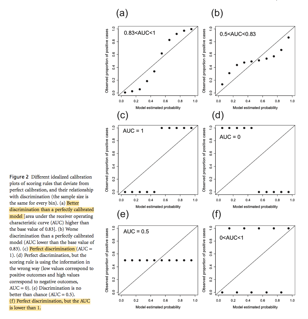
Jiménez‐Valverde et. al. thus examined how changes in the distribution of probability of occurrences make discrimination capacity is a context-dependent characteristic. Through simulation, they found that a well-calibrated model, where the probability of randomly chosen positives have higher S then randomly chosen negatives (P) is equal to S, will not attain high AUC value, which is 0.83. and confirmed that discrimination depends on the distribution of the probabilities. Figure 2 shows some extreme cases demonstrating trade-offs between discrimination capacity and calibration reliability. When a model is well calibrated, dots should line up along the solid line.

Screen Shot 2016-02-17 at 12.05.25 PM

This paper not only well explained the difference between discrimination and calibration and why the increase of one compromises another, it also pointed out two implications in the field of SDM: first, it explains the devilish effect of the geographic extent, which is the reason for the negative relation between the relative occurrence area and discrimination capacity; second, discrimination may not be used to compare different modeling techniques for the same data population and to generalize conclusions beyond that population. It is noteworthy to aware limitations and conditions when evaluating our own models. One practical way is to not report AUC alone, but also be accompanied with information about the distribution of scoring system and, if possible, the model calibration plots.

AUC: a misleading measure of the performance of predictive distribution models

Lobo, J. M., Jiménez-Valverde, A., & Real, R. (2008). AUC: a misleading measure of the performance of predictive distribution models. Global Ecology and Biogeography, 17(2), 145–151. http://doi.org/10.1111/j.1466-8238.2007.00358.x


With the increase in the use of predictive distribution models, especially with regards to species niche modeling, many are turning to the the area under the receiver operating characteristic curve (AUC) to assess the predictive accuracy of the models. Lobo et al have five main issues with the use of AUC in this manner. According to Lobo, AUC…

1) is insensitive to transformations of predicted probabilities, if ranks are preserved, meaning that models that are well fit may have poor discrimination and vice versa
2) summarizes test statistics in areas of extreme false-positive and –negative rates that researchers are rarely interested, leading the authors to suggest partial AUC
3) weights omission and commission the same. In the case of presence-absence data, false absences are more likely than false presence data, therefore their respective errors are not equal
4) plots do not describe the spatial distribution of errors, which would allow researchers to examine whether errors are spatially heterogeneous
5) does not accurately assess accuracy if the environmental range is larger than the geographical extent of presence data, as is the case for most SDM predictions

Additionally, AUC is often used to determine a ‘threshold’ probability of species distribution when converting a SDM to a binary, in spite of the fact that a ‘benefit’ of AUC is it is independent of the chosen threshold, and its corresponding subjectivity. The only instance in which the authors encourage use of AUC is in distinguishing between species whose distribution is more general (low AUC score) vs restricted. In order to combat the failings of AUC, Lobo et al suggest that sensitivity and specificity also be reported and that AUC only be used to compare models of the same species over an identical extent. I think another important point to include would be the quality of data. A cause of several of these problems is the bias of absence data in species distributions, and extra effort to combat this bias and ensure more complete presence-absence data sets would reduce the bias introduced by AUC.

What do we gain from simplicity versus complexity in species distribution models?

Merow, Cory, et al. “What do we gain from simplicity versus complexity in species distribution models?.” Ecography 37.12 (2014): 1267-1281.

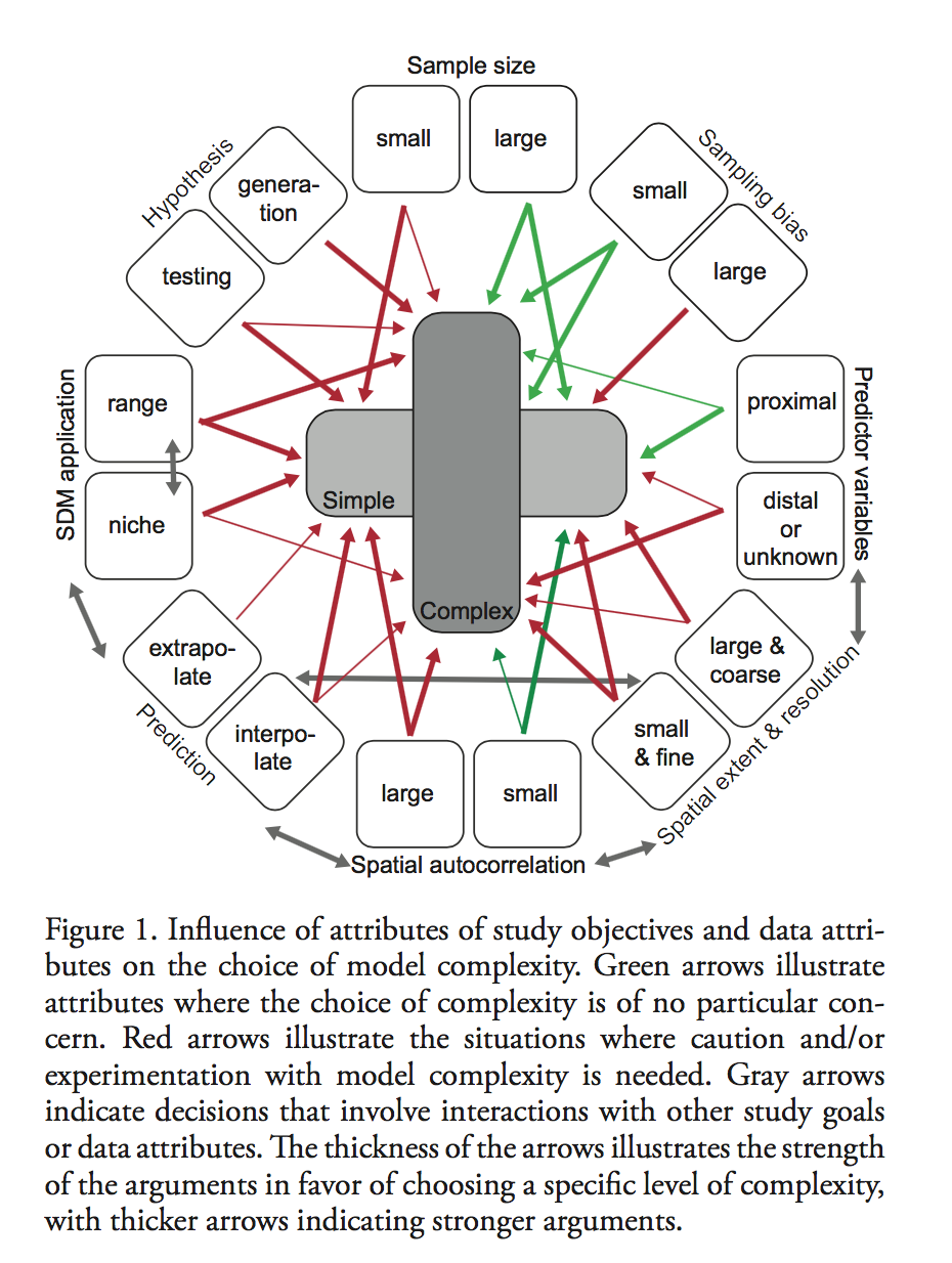
A variety of methods can be used to generate Species distribution models (SDMs), such as generalized linear/regression models, tree-based models, maximum entropy, etc. Building models with an appropriate level of complexity is critical for robust inference. An “under-fit” model will introduce risk of misunderstanding factors that shape species distribution, whereas an “over-fit” model brings risks inadvertently ascribing pattern to noise or building opaque models. However, it is usually difficult to compare models from different SDM modeling approaches. Focusing on static, correlative SDMs, Merow et. al. defined the complexity for SDM as the shape of the inferred occurence-environemnt relationships and the number of parameters used to describe them. By making a variety of recommendations or choosing levels of complexity under different circumstances, they developed negeral guidelines for deciding on an appropriate level of complexity.

There are two attributions determining the complexity of inferred occurrence-environment relationships in SDMs: the underlying statistical method (from simple to complex: BIOCLIM, GLM, GAM, and decision trees) and modeling decisions made about input and settings. As for modeling decision, larger numbers of predictors are often used in machine-learning methods instead of traditional GLM. Incorporating model ensembles and predictor interactions will also increase model complexity.


Screen Shot 2016-02-10 at 1.39.59 PM

Figure 1 summarized their finding in terms of general considerations and philosophical differences underlying modeling strategies. They suggested that before making any decisions on model approaches, researchers should experience both simple and complex modeling strategies, and carefully measure their study objectives (Niche description or range mapping? Hypothesis testing or generation? Interpolate or extrapolate? ) and data attributes ( sample size, sampling bias, proximal predictors and distal ones, spatial resolution and scale, and spatial autocorrelation). Generally speaking, complex models work better when objective is to predict, and simpler models are valuable when analyses imply only certain variables are needed for sufficient accuracy. Finally, they concluded that combining insights from both simple and complex SDM approaches will advance our knowledge of current and future species ranges.

Relating this paper with the Breiman paper, Merow et. al. regarded data modeling models simpler than algorithmic models, which are usually semi- or fully non-parametric. But they also acknowledged that this conception is rather relative: the interpretability of complex models is not necessarily difficult, and the complexity can still identify simple relationships. However, it can be seen that Merow et. al. regarded interpretation of models one of the goals of modeling. They think there is no absolute situations that simple models or complex models violate the nature of science, but their merits are more case-dependent. I think the combing of simple and complex models, as Merow et al suggested, is the trend of statically modeling, and Breiman maybe over-emphasized the distinctions between the two cultures in modeling world.

Looking Forward by Looking Back:
Using Historical Calibration to Improve Forecasts of Human Disease Vector Distributions

Sohanna, A. & Thomas, K., 2015. Looking Forward by Looking Back: Using Historical Calibration to Improve Forecasts of Human Disease Vector Distributions. Vector-Borne and Zoonotic Diseases, 15(3), pp.173–183. link

With rising concerns about how environmental change impacts disease vector distributions, many studies aim to predict future vector distributions under varying climate change scenarios using information available at present time. Many types of species distribution models enable us to produce highly accurate present-day data on vectors of disease. However, when trying to forecast or ‘hindcast’ species distributions many models are never validated with independent data on past or separately observed distributions. This review paper focuses on (1) methods of validation for present day spatial models, (2) how these models should be projected into the future, and (3) introduce the method of historical calibration for validation. The authors explain three methods of validation for present day spatial models and their limitations: the commonly used split-data approach (training & test data), independent dataset validation (geographically or temporally distinct data sets for validation), and validation via occurrence of disease in reservoir species. Next, the authors reviewed the use of GCMs to model future climates and their limitations including ignoring biological processes and non-linearities as well as using constant change environmental increments without setting theoretical limitations. Lastly, they suggest that historical calibration, a validation method rooted in macroecology, is more temporally transferrable in the context of projecting vector distributions and when coupled with reliable ensemble models could reduce current shortcomings in forecasting species distributions.


Modelling ecological niches with support vector machines

JM Drake, C Randin, and A Guisan. 2006. “Modelling ecological niches with support vector machines” J of Applied Ecology. 43, 424-432.

Machine learning approaches get around common obstacles to species distribution modeling (autocorrelated data, presence-only data, etc.), but are relatively recent tools for species distribution modeling. The authors promote and demonstrate the use of Support Vector Machines (SVMs) to model ecological niches, using 106 alpine plant species as a case study.

Benefits of SVM approach

1. Not based on statistical distribution (no independence requirement)
2. SVMs are a one-class approach, simplifying the classification problem (presence-only)
3. Fewer tuning parameters, and deterministic results (model will always converge to same solution given a dataset)
4. Not many observations needed (n=40). Not sure how this compares to other methods though.
5. SVMs are cross-validated
6. SVM and niche both defined as boundary in hyperspace, so using SVM is on firm conceptual ground

The authors test 3 different methods that used dimensionality reduction or variable removal. SVMs performed comparably to MaxEnt, ENFA, and other methods (they didn’t examine all methods on their data, but compared the accuracy they obtained with other published studies on different systems). SVMs without any feature reduction or variable transformations performed the best.

Do they? How do they? WHY do they differ? On finding reasons for differing performances of species distribution models

Elith, J., & Graham, C. H. (2009). Do they? How do they? WHY do they differ? On finding reasons for differing performances of species distribution models. Ecography. http://doi.org/10.1111/j.1600-0587.2008.05505.x

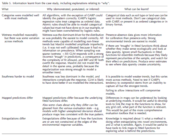
With the expansion of SDM has come an increasing emphasis on machine-learning models, however there are few resources available for newcomers to help guide which models to choose for which application, or end goal. As a first step in creating such a guide, Elith & Graham use a simulated plant presence-absence data set and assessed the success of five algorithms to achieve three common goals in SDM: 1) understanding the relationship between a species and its environment, 2) creating a map of habitat suitability, and 3) extrapolating to new environmental conditions. The five algorithms were a generalized linear model, boosted regression trees, random forests, MaxEnt, and GARP, the last two using presence-only data. They compared each algorithm’s performance for each of the three applications of SDM, using four different measures of statistics. Their results are summed up in the table below, and I’m not going to rehash them here. An important conclusion they drew from their comparisons, however, are that the researcher must have an understanding of the algorithm they are using and the ecological background of their system in order to choose the best model for their application and system. For example, GARP does not model categorical variables well, and presence only models may not be well calibrated depending on the range of suitability. I found it interesting that, even though these algorithms still represent a ‘black box’, a user’s understanding of their strengths and weaknesses will allow the user to better interpret the somewhat subjective output in choosing a model of ‘best fit’ for their chosen goal.

Screen Shot 2016-02-08 at 6.35.33 PM

In defense of ‘niche modeling’; ‘Niche’ or ‘distribution’ modeling? A response to Warren

These papers discuss and argue the terminology used to describe the process of determine where species are able to inhabit.  Specifically the use of the terms Ecological Niche Models and Species Distribution Models to describe the techniques used to determine where or potentially where species are able to inhabit.

Warren (2012) criticizes the “loss” of the niche in the terminology.  While he sympathizes that many of these models are trained using data that only comes from the distribution of a species, he also argues that the underlying assumption of these models is that they are estimating the niche. The argument that these environmental predictors have some effect on biological processes of the organism and that often these models omit processes (e.g. dispersal).  Here, he defines the niche as the “conditions within which the species can survive and reproduce”. He suggests we continue to acknowledge the conceptual framework being used and the we are attempting to estimate the niche in our research.

In a response to Warren, McInerny and Ettienne (2013) defend the position of using ‘distribution’ to describe the techniques.  They criticize his definition (even the definitions he provides, pointing out that he invokes two ones)  of niche saying it constrains the selection of predictor variables to ones that are only biological.  However, they point out that these problems have also been considered with the SDMs through parameter selection, model structure, and functional forms.  Lastly, the point out that other words could also be used to describe these models (“habitat suitability”, “bioclimate envelopes”, “resource selection”) but they stand by the choice of the neutral words “species distribution modeling”.

Warren, D. L. 2012 In defense of ‘niche modeling’. Trends Ecol. Evol. 27, 497–500. doi:10.1016/j.tree.2012.03.010

McInerny, G. J. & Etienne, R. S. 2013 ‘Niche’ or ‘distribution’modelling? A response to Warren. Trends Ecol. Evol. 28, 191–192. http://dx.doi.org/10.1016/j.tree.2013.01.007

Scale-dependent role of demography and dispersal on the distribution of populations in heterogeneous landscapes


Motivation: Both dispersal and local demographic processes shape the distribution of the population among varying habitat qualities. However most theories, experiments, and field studies have focused on dispersal.  The authors attempt to show how both dispersal and demographic processes shape a population’s distribution, and when either mechanism is more important.

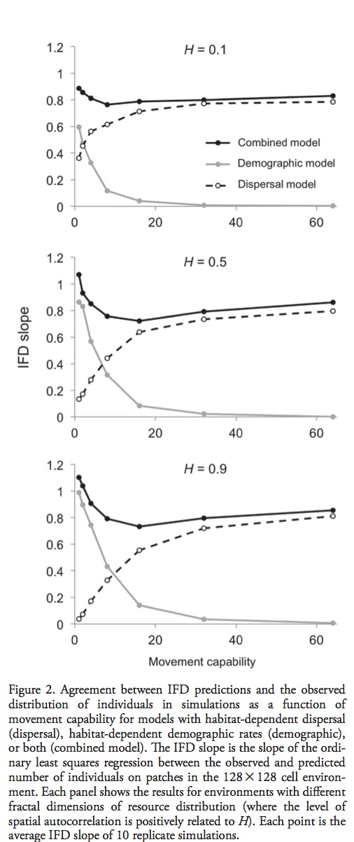
Population dynamics were primarily explained via demographic processes, while distribution was a function of dispersal process. These authors would also like to bring in the ideal free distribution (IDF) theory to explain population distributions.  IDF  predicts that individuals will be distributed among patches of different quality so that the fitness of individuals in different patches is equalized – individuals can’t improve fitness by moving to another patch. As an aside, given that the underlying theory requires individual choice of patch occupancy this work is only appropriate for populations that can actively choose how they are dispersed or move.  The IDF can arise from 2 possible mechanisms: 1) dispersal, where individuals use information about habitat quality to make movement decisions, or 2)  demographic processes where the habitat quality experienced by individuals affects demographic rates.

Methods:  The authors explore the 2 mechanisms that lead to IDF by extending a individual-based model of habitat dependent dispersal, growth, reproduction, and survival of individuals. All simulations wer done on a 128 x 128 cell grid. Each  grid/habitat patch had its own logistically growing resource, and patch quality differed by the carrying capacity of this resource. To examine the relative effects of dispersal and demography, the model simulations were run with only habitat dependent dispersal, habitat dependent demography, or both.   This was done by varying 2 traits: the maximum dispersal distance (M) and the spatial scale of resource heterogeneity (H).

Wk4Fig 2


Results: When both habitat dependent dispersal and demography were included in the simulation population distributions closely matched IFD predictions.   Simulations of populations with only demographic processes (i.e. Dispersal only) were overabundant in low-quality patches and under abundant in high-quality patches resulting in low correlation with IFD predictions. This effect was exacerbated in environments where the spatial scale of resource heterogeneity was large. When habitat quality influenced demographic rates (but dispersal was random), the effect of scale on IFD  was reversed – highly mobile populations were sub optimally distributed with respect to habitat quality, reducing the scale of resource heterogeneity only exacerbated the trend.

Take-home: Pulliam demonstrated the need to include passive dispersal processes when describing population distributions, Martin et al.  has demonstrated the need to include dispersal and demographic processes of populations with active dispersal. Spatial scales that limited the resource matching capacity of one process coincide with those that promoted the resource matching capacity of the other process.


Martin, Benjamin T., et al. “Scale‐dependent role of demography and dispersal on the distribution of populations in heterogeneous landscapes.”Oikos (2015).  doi: 10.1111/oik.02345

The vulnerability of species to range expansions by predators can be predicted using historical species associations and body size

The vulnerability of species to range expansion by predators can be predicted using historical species associations and body size. Declines in abundance in local extinctions are the direct consequence of climate exceeding physiological tolerances in addition to the indirect consequences of climate change on species interaction. These indirect impacts of climate change and biodiversity are more difficult to predict or observed when compared to the physiological impacts.

Species ranges have changed at variable rates under climate change, potentially making novel ecosystems. However, species expanding their range can encounter resident prey, predators and competitors that were present in their historical range (i.e. species historically occurred in some patches). The ecological niche concept has been used to understand patterns of co-occurrence and species interaction; this could also be a useful tool to protect the indirect impacts of climate change.

Here, the authors suggest using species associations and body size as a simple measure of the impacts of species introductions facilitated by climate change. Negative associations can indicate strong ecological interactions including competitive exclusion, predation or it could indicate different abiotic requirements. Functional traits often mediate the strength of species interactions – which can be used to infer niche differences. Body size is correlated with many functional traits (i.e. reproductive rate, dispersal ability, diet breadth and or predation). Increased differences in body sizes would indicate decreased competition, while the ratio of predator to prey body size indicates strength of predation.

The authors hypothesize that pairwise species associations and body size can predict the relative risk imposed on resident species by predators whose ranges are expanding. They focus centrarchid predators undergoing range expansion in the Great Lakes region. This expansion is expected to be problematic since these predators are not often found in smaller lakes with the potential prey species. The question then becomes whether this negative species associations are good predictors of vulnerability, and how resident species body size impacts the risk associated with additional predators.

Methods: The data set consisted of 1551 links with paired historical and contemporary species samplings. A total of 106 fish species were observed which was then used to create presence absence data pairs in 2 x 2 contingency tables. The Phi– coefficient was calculated for these 2 x 2 tables (range from -1, 1) the relative risk ratio was then calculated on the tally of lakes where the resident species was absence after the introduction of the predator.

Results:  Centrarchid introductions significantly increase the likelihood of some prey species loss, while protecting loss of native centrarchids based on introduction data. Historical species associations were a strong predictor of the introduced species’ impact. Additionally, resident species total length was a significant indicator of the relative risk ratio.

Take home:  Traits mediate species interactions, and body size is an easily measurable trait that is correlated to many other traits in fish species. Body length and historical species associations can be used to forecast the impact of introduced species on the native species under climate change.

Given that fish can have convoluted food webs, using body size as a proxy of competition and predation seems like a very elegant solution.


Alofs, Karen M., and Donald A. Jackson. “The vulnerability of species to range expansions by predators can be predicted using historical species associations and body size.” Proc. R. Soc. B. Vol. 282. No. 1812. The Royal Society, 2015. http://dx.doi.org/10.1098/rspb.2015.1211