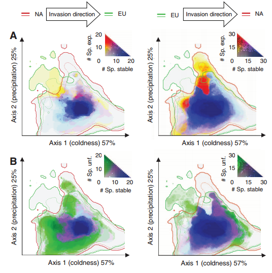
Species may be able to shift their climatic niche requirements according to some researchers, while most models of diversity as a function of global change assume a constant climatic niche for a given species. This is especially the case in species invasions, where the species may be able to exist in climates different from the native range. The authors examined 50 invader plant species in North America and Eurasia in order to quantify the degree of niche expansion, niche overlap, and niche unfilling (species only partially fills its native niche in the invaded range). They found niche conservatism in 46% of the plant species, suggesting that plants largely occupy similar niches in their invaded range. Further, the authors found that when niche expansions were present, 14% of these species show greater than a 10% niche expansion, which they argue is rather low. Niche unfilling was rather common (48% of species), though they don’t discuss the influence of dispersal limitation or the influence of time since invasion on this result. One would think that recent invaders that haven’t had time to disperse (or those under active control) would not have time to reach the extent of their niche, which would appear as niche unfilling compared to their niche in the native range. In their supplement, the authors detail how they calculated the E-space used to quantify niche overlap (a standard PCA whose first two axes explained 82% of the variation in 8 variables including degree day, evapotranspiration coefficients, temperature and precipitation).
Category: Student summary
Facilitation and the niche: implications for coexistence, range shifts and ecosystem functioning
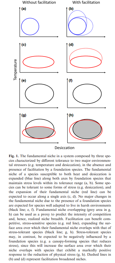
The original description of the niche purposefully excluded the impact of species interactions for niche determination. In a more applied context, several authors have included species interactions, specifically negative interactions, in determining a species niche or geographic range. Here, the authors consider the effect of facilitatory interactions on the expansion of the niche. An example would be if the presence of another species created habitat necessary for the colonization of a secondary species, such as the case with woodpeckers facilitating the presence of tree hole dwelling insects. Species interactions could create suitable environments (e.g., microhabitat variation; see Chesson (2000)) or provide access to a resource that could enable persistence. The authors argue that the introduction of a facilitatory species could result in a niche shift of a focal species in E-space (as in Figure 1). The authors also discuss the role of coexistence when competing species are both responding to a facilitatory species. They argue that niche broadening as a function of facilitation may promote exclusion of one of the species, as niche broadening may put two species in competition where they previously weren’t. This will only be a big issue when fitness differences are large.
Chesson, P. (2000a) Mechanisms of maintenance of species diversity. Annual Review of Ecology and Systematics, 31, 343–366
Environmental data sets matter in ecological niche modelling: an example with Solenopsis invicta and Solenopsis richteri
Authors: Peterson and Nakazawa
DOI: http://10.1111/j.1466-8238.2007.00347.x
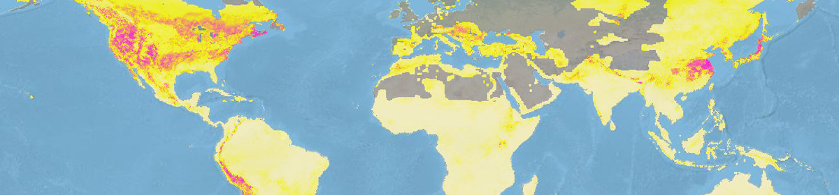
This study highlights the potential effects environmental data can have on model results. The study system selected by researchers was assumed to be a matured species invasion of fire ants where experts were confident that the invading species was approaching its range limit. Researchers compared six different environmental data sets with a genetic algorithm rule-set prediction (GARP) for model development. The different types of rainfall data sets considered were the following: WC1, WC2, IPCC, CCR, and NDVI. GARP operates by sampling available occurrence points (with replacement) to build a population of a set number of presence points, and then an equal number of sampled points of no occurrence. Both sets of occurrence/no-occurrence are then divided equally into training and testing data sets. A drawback to this study is that comparisons are made only qualitatively by depicting predictive differences through mapping, and no quantitative measure of model performance is provided. It is clear from the results offered that different environmental data sets can yield differences in model prediction, yet the authors provided little speculation on possible reasons for such differences.
Vacated niches, competitive release and the community ecology of pathogen eradication
Lloyd-Smith JO. 2013 Vacated niches, competitive release and the community ecology of pathogen eradication. Phil Trans R Soc B 368: 0120150. http://dx.doi.org/10.1098/rstb.2012.0150
This article reviews whether it is sensible to consider the niche left behind when a pathogen is eradicated, and to worry about the risk that this niche will be recolonized by another pathogen causing a similar disease. This topic is highly controversial in the epidemiological literature regarding he merits of eradication. Lloyd-Smith proposes the term ‘vacated niche’ to describe the pathogen niche left behind following a successful eradication effort and evaluates evidence claiming that vacated niches can alter the epidemiology of the surrounding community of pathogens. Potential mechanisms of competitive release or evolutionary adaptation can elevate the health burden from other pathogens (i.e. resulting in increased incidence of another pathogen). However, he emphasizes that a vacated niche will not necessarily cause emergence of a replacement pathogen, or that any such pathogen will have similar disease characteristics to the eliminated one. He concludes that the vacated niche is an opportunity for other pathogens, but many factors will determine whether and how they may capitalize on it. This article is an expansion to the ecological discussion of whether empty niches actually exist and it is interesting to think about how these concepts would lend themselves to invasive species and/or local species extinctions.
Demographic compensation among populations: what is it, how does it arise and what are its implications?
Villellas, J., Doak, D. F., García, M. B., & Morris, W. F. (2015). Demographic compensation among populations: what is it, how does it arise and what are its implications? Ecology Letters, 18(11), 1139–1152. http://doi.org/10.1111/ele.12505
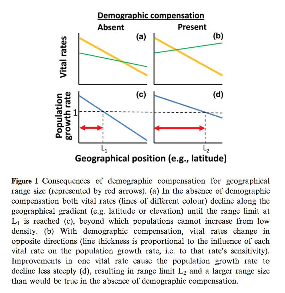
A common assumption in the analysis of species distributions across an environmental gradient are that vital rates decline across the gradient as they approach the range limit. Villellas et al. aimed to investigate an opposing theory, demographic compensation (DC), in which mean population vital rates change in opposing ways across spatial or environmental gradients. Using a randomization procedure, they tested for the presence of DC across 26 plant demographic studies, based on the assumption that DC would lead to more negative correlations among vital rates than expected by chance. They found both that there were more positive and more negative correlations than expected by chance, suggesting that the overall tendency is for vital rates to respond similarly, but that DC is a phenomenon that does exist. Investigating further, this pattern was driven by fecundity and recruitment rates, which had the highest proportion of negative correlation amongst vital rates and to which the population growth rate had high variance and sensitivity, respectively, evidence that DC acts by influencing vital rates as different life stages. For those studies that showed evidence of DC, another randomization procedure was done to compare the variation of population growth rates with a nd without DC, finding that DC halved the variance in population growth rates. This has important implications for SDM, as high growth rate variation at the range limits of species distributions can lead to a higher rate of stochastic extinctions, perhaps influence presence data and the probability of persistence in these limits. If we are to believe that DC is at play, however, there will be less variation at the range limits, implying that the ‘e-space’ may be closer to Hutchinson’s binary persistence-extinction demarcations than originally thought.
Five (or so) Challenges for Species Distribution Modeling
The authors present 5 challenges for SDM. By confronting these models, we should be able to generate better and provide a better understanding of these models.
- Clarification of the niche concept: The authors suggest a diversion from the Hutchinson definition of the niche (n-dimensional hyper-volume of environmental variables) to more of a Grinnellian definition: the set of environmental conditions at which the birth rate of the population is greater than or equal to the death rate. They also point out the need for the clear(er) distinction between potential habitats for species (ranges/areas that the conditions are “right” for a species to inhabit) and potential geographic distributions of species (incorporates spatial factors such as dispersal)
- Improved designs for sampling data for building models: Models are sensitive to bias. Subsampling datasets are likely to remove or reduce biases. A (more expensive) alternative is to target specific, strategic additional sampling locations.
- Improved parameterization strategies: Different parameterizations of models can result in vastly different projections of species distributions. We to better understand why and when different parameterizations of the same technique provide different results.
- Improved model selection and predictor contribution: There are many different strategies that can be used to compare different models. However, finding the individual contribution of each predictor is a more difficult problem. Further testing of proposed solutions provided by the authors is needed.
- Improved model evaluation strategies: Evaluation of models can be discussed in the light of three different implementations: explanation, understanding and prediction. Typically modelers use the “wrong” evaluation tool outside of the scope of their goal or question. They present two different forms of evolution: verification (projecting using an new/independent set of data) and validation (maximizing the fit to training data).
Araújo, M. B. & Guisan, A. 2006 Five (or so) challenges for species distribution modelling. J. Biogeogr. 33, 1677–1688. (doi:10.1111/j.1365-2699.2006.01584.x)
The Combined Use of Correlative and Mechanistic Species Distribution Models Benefits Low Conservation Status Species.
Rougier, T., Lassalle, G., Drouineau, H., Dumoulin, N., Faure, T., Deffuant, G., Rochard, E. and Lambert, P. 2015. The Combined Use of Correlative and Mechanistic Species Distribution Models Benefits Low Conservation Status Species. Plos One, 10, 21. DOI: 10.1371/journal.pone.0139194
The spatial distribution of species suitable habitat has typically been projected using correlative Species Distribution Models (SDMs). Now increasing evidence suggests that rapid evolutionary change, dispersal, spatial structure of the environment, and population dynamics are also important for determining future species ranges. This paper seeks to develop a framework for joint analysis of correlative and mechanistic SDMs in order to increase the robustness of model-derived conclusions and aid resource managers involved in species conservation planning. Two previously constructed models, one correlative and one mechanistic, were used along with biological data collected from the literature EuroDiad 3.2 database which contains distribution information for European diadromous fishes from 1750-2010. Due to computational constraints a subset (73 of the 197 river basins included in the database) were used to predict species distribution using the mechanistic model. Both the correlative and predictive model correctly predicted historical presence data (before 1900) for the river basins used, though they did not predict absences within the historical data set well. In this case both models predict a high probability of self-sustaining populations of allis shad under moderate and pessimistic climate change models. This study concludes that when available predications from correlative and mechanistic modelling should be utilized in a complementary way to help guide conservation efforts in light of climate change. While the paper does provide a framework for jointly analyzing a correlative and mechanistic distribution model it only briefly addresses the issues encountered regarding the increased intensity in the amount of data and computational power required to utilize the mechanistic SDM. For now, it may be a rare case when correlative and mechanistic SDMs can be used in a complementary way as presented in this paper.
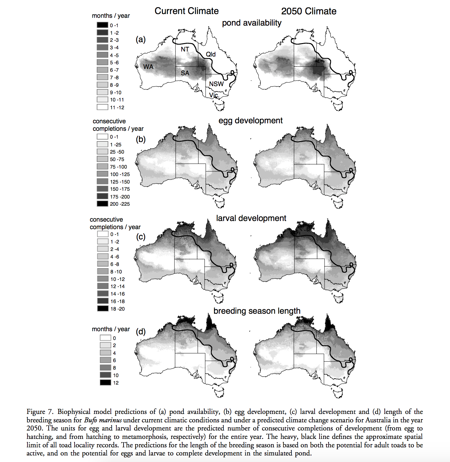
Modelling species distributions without using species distributions: the cane toad in Australia under current and future climates
Almost all approach for GIS-based distribution modeling depend in some way on species occurrence data. In range-shifting species, however, the correlative approach usually requires extrapolation to novel environments, which could lead to erroneous predictions. Kearney et. al. used an alternative approach with emphasis on the ecology of organisms based on ecophysiology and organism traits, which is independent from species current distribution. They used fine-resolution spatial dataset together with a set of biophysical and behavioral models to make the predictions of Cane Toads distribution under current and future climate in Austrilia, assessing the direct climatic constraints on their ability to move, survive, and reproduce. The results show that the current species range can be explained by thermal constrains for the adult stage and water availability for the larval stage. Their research provided a framework showing trait-based approaches can be used in investigates the range limits of any species by quantifying spatial variation in physiological constraints and therefore defining regions where survival is impossible. They claimed that mechanistic approaches have broad application to process-based ecological and evolutionary models of range-shift. In my opinion, an effective mechanistic model depends on sophisticated observational or empirical data to from the mechanism of the target organism, which maybe not that easy to obtain for all kinds of species. In addition, researchers could never capture all factors for the fundamental niche. The way Kearney et. al. addressed this problem is by identifying areas outside the niche and to locate impossible areas for the organisms. Therefore, their predicted areas are less restricted than the actual range.
Kearney, M., Phillips, B. L., Tracy, C. R., Christian, K. A., Betts, G., & Porter, W. P. (2008). Modelling species distributions without using species distributions: the cane toad in Australia under current and future climates.Ecography, 31(4), 423-434. DOI: 10.1111/j.0906-7590.2008.05457.x
Modelling ecological niches with support vector machines
Drake, Randin, & Guisan (2006) tested the method of support vector machines (SVMs) to map ecological niches using presence-only data for 106 species of woody plants and trees in a montane environment with nine environmental covariates. Support vector machines (SVMs) utilize machine-learning techniques designed to model one type of data only by finding statistical patterns and then removing outliers to estimate the support of high-dimensional distributions. The support of the distribution of a species’ environmental requirements is analogous to Hutchinson’s ecological niche concept. In situations with presence-only, SVMs are simpler (and differ from other methods) because they eliminate the requirement for pseudo-absence data. This paper compares three ways of using the SVM approach: (1) using no pre-processing or data reduction to the nine environmental covariates, (2) pre-processing training data using k-whitening, and (3) restricting covariates by removing highly correlated environmental variables. They found that method 1 resulted in models with the highest recall (ratio of number of correct predictions to total number of observations) and lowest false positive rate. Method 3 performed the worst overall, suggesting that useful information about ecological niches can be obtained by the inclusion of more environmental variables, even if they are highly correlated. Additionally, they found that the SVM method required approximately the same amount of observations as comparable methods, and resulted in similar AUC values for prediction. This paper helped to develop a background understanding of the literature on machine-learning techniques to model presence-only vs. presence-absence data and how the aforementioned methodological differences determine whether a species’ fundamental or realized niche is being modeled.
Drake, J.M., RANDIN, C. & GUISAN, A., 2006. Modelling ecological niches with support vector machines. Journal of Applied Ecology, 43(3), pp.424–432.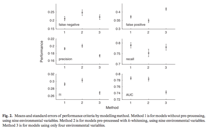
Modeling the spatial distribution of two important South African plantation forestry pathogens
Van Staden et al. (2005) used a bioclimatic species distribution model to find the broad habitat distribution and potential distribution of two fungal pathogens of commercially important tree species, pines and eucalyptus, in South Africa under varying climate change scenarios. The distribution and infectivity of both pathogens are affected by certain climatic parameters (e.g. hail damage, high rainfall, and humidity) and climate change impacts these variables. Fungal incidence data for the study consisted of 87 confirmed reports of S. sapinea and 17 reports of C. cubensis and climate data for the area were obtained from existing literature and a digital elevation model for South Africa. Climate data included five variables: altitude, average rainfall of driest and wettest month, and average temperature of hottest and coldest month. The bioclimatic model incorporated these five variables, created a multidimensional scatter plot using for each variable for each grid cell in South Africa (11,800 total), generated matrix of covariates for each cell, and then transformed that matrix into a probability of occurrence for each fungus for each cell. Consequently, they were able to identify core-risk regions for both fungi, and found that those regions included major commercial forestry plantations. They report this as the first study to utilize a bioclimatic model to predict the distribution of economically relevant pathogens for eventual use in decision support systems for forestry management. This study could be improved by increased data on the fungus (more than 100 counts of each) and potentially exploring the variation in predictions generated by the model. It would be interesting to explore different combinations of variables or data points and how the predications would change based on each combination.
van Staden, V. et al., 2004. Modelling the spatial distribution of two important South African plantation forestry pathogens. Forest Ecology and Management, 187(1), pp.61–73.