Fine-Scale Predictions of Distributions of Chagas Disease Vectors in the State of Guanajuato, Mexico

, , , , , , , ,

http://dx.doi.org/10.1093/jmedent/42.6.1068

Many species distribution models (specifically regarding models for the triatomine vector) are conducted at large geographical scales whereas smaller local scales may be more useful in understanding significant drivers of specific triatomine species distributions and thus a more localized disease risk. Lopez-Cardenas assesses a fine-scale distribution (“ a landscape view”) for 5 triatomine species: Triatoma Mexicana, T. longipennis, T. pallidipennis, T. berberi, and T. dimiata by geo-referencing collection localities and using ecological niche modeling with an evolutionary-computing approach. Triatomine species were collected from the field from 201 communities within Mexico. Risk for disease transmission was also assessed from niche mapping results. Predictor variables included the use of multi-temporal, remotely sensed environmental data sets as surrogate for climate data which permits fine-scale predictions across landscapes since climatic monitoring stations are too sparse to permit development of fine-scale climatic maps. Triatomine occurrence points, were used for each triatomine species and processed in the model GARP to determine species ecological niche.  Data were separated into training and testing data and rule variable selection was developed through an iterative selection process. 100 models were generated from the same selective process and the best models were chosen based on ideal omission and commission errors. Chi-squared test was used to compare observed success in predicting distributions of test points with those expected under random models. Results from using GARP has suggested which species provide a greater risk to human health based on their distribution patterns in Mexico. In retrospect, the quality of data they collected seemed ideal for any vector-presence study I’m just curious why they would use occurrence only models such as GARP when they have a good idea of species absence data as well. Perhaps it would be better to use presence-absence models in this situation because of the quality and credibility of their data, and therefore are more likely to have true absences.



Biotic interactions boost spatial models of species richness

Integrating biotic interactions into the framework of species richness models has been a suggested to improve the performance of both species distribution models.  The authors seek to use biotic variables in two species richness modeling frameworks.  Stacked species distribution models (SSDM) fit separate species distribution models then blindly stacks the results of the predicted occurrences to calculate the species richness.  The macroecological models (MEM) do not use the information provided by species identity and community composition to estimate the species number using environmental conditions.  This model assumes species richness is limited by environmental conditions. Using these two models, three different groups of taxa (vascular plants, bryophytes, and lichens) used to examine the effect of integrating biotic variables.

When comparing the results of the models using biotic interactions to models with only climatic and abiotic, biotic models performed consistently better.  Both modeling frameworks and all taxonomic groups using biotic interactions had a lower bias and increased predictive power. These results highlight the importance of using biotic predictor variables in not only species richness models but also single species distribution models.

Mod, H. K., le Roux, P. C., Guisan, A. & Luoto, M. 2015 Biotic interactions boost spatial models of species richness. Ecography (Cop.). 38, 913–921.

Mapping large-scale bird distributions using occupancy models and citizen data with spatially biased sampling effort

Higa, M., et al. (2015). “Mapping large-scale bird distributions using occupancy models and citizen data with spatially biased sampling effort.” Diversity and Distributions 21(1): 46-54.

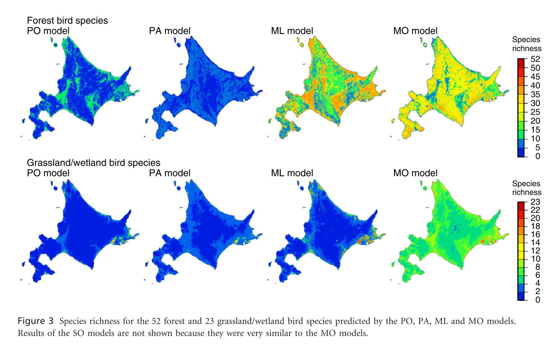
Citizen science data offers the ability to collect large amounts of species distribution data that would be impossible for a researcher to gather otherwise. This data can, however, suffer from issues of inconsistent data quality across the range (because of inconsistency in the expertise of citizens) and spatial sampling bias. The authors consider multiple SDM methods and their performance when applied to an aggregated data set collected by professionals and citizens with spatially biased sampling effort. Records of bird species presences were sorted into 4 categories: point census by experts, line census by experts, observation with other methods by experts, and observation with other methods by citizens. Environmental covariates were land cover and elevation. Models employed were presence-absence (PA) or presence-pseudoabsence (PO) (depending on available data) logistic regression, MaxLike, and two types of occupancy models. One type of occupancy model analyzed each species individually (SO) while another analyzed multiple species in the same model (MO). Both of these models depend estimation of latent occupancy (a Bernoulli variable) and detection/non-detection (a Bernoulli variable based on occupancy and observation probability from detection/non-detection data. The SO models for 18 forest bird species and two grassland/wetland bird species did not converge. Detection probabilities for all species were below 1 and differed by observation type (line census by experts>other methods by citizens and point census by experts>other methods by experts). Probability of presence for forest species decreased with forest area for PO and ML models while it increased with forest area in PA and especially occupancy models. Grassland/wetland species probability of presence increased with grassland and/or wetland area across all models though species richnesses predicted by PA, PO, and ML were lower than occupancy models. Both types of occupancy models (SO and MO) generally agreed. The authors claim that this work demonstrates the weakness of MaxLike and presence-only logistic regression in the face of spatial sampling bias. They put forward occupancy models that explicitly model detection as an easier and equally effective method as, if not a more effective method than, accounting for bias through similarly biased absence data (PA). Though this study lacks any actual evaluative measures (beyond the assumption that forest species should be more likely to occur in larger forests), the process of occupancy modeling seems nonetheless very promising and should certainly be tested more broadly.


higa figure

Empirical evidence for source-sink population: a review on occurrence, assessments, and implications

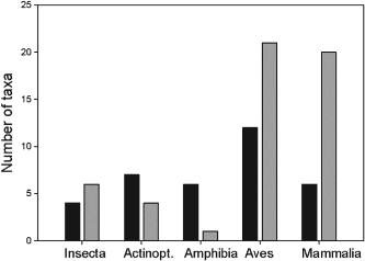
The paper provides a review and synthesis examining the occurrence of source and sink populations in the literature.  Pullman (1988) stated that sink habitats would need inputs from nearby sources to persist in the landscape. As the need for conservation planning increases, a better understanding of what may affect the presence of source and sink habitats is crucial. Prior to performing the analysis, the authors provide systematic and biological predictions about what may influence source and sink population occurrence.

Methodological:

  1. There will be less evidence for source populations then sink population.
    1. The authors were correct in this prediction there was more evidence for sink populations across taxa (however, this finding was not significant, p=0.059).

brv12195-fig-0002 brv12195-fig-0002

Black bars represent source populations. Grey bars are sink populations.

  1. The spatial scale of the studies will affect the detection/occurance of source and sink populations.
    • Was not supported.
  2. When several, i.e. more than a few(?), local populations are considered, there will be more evidence for source populations.
    • Was not supported.
    • The authors comment that more demographic data should be record when examining populations (i.e. fecundity/mortality, immigration/emmigration).

Biological

  1. More sources are expected when the local population is stable or increasing. Sinks when the local population is decreasing.
    • Was not supported.
  2. Sources are expected in resident species rather than migratory.
    • Was not supported.
  3. Low-dispersal ability species are expected to have more sources than high dispersal ability species. Also, high dispersing species are expected to have more sinks than limited dispersal species.
    • Was not supported.
  4. Well-connected local populations are expected to have more sources.
    • The prediction was supported, local populations that were well-connected were more likely to have sources. Immigration between may prevent stochastic/demographic extinction of patches.
  5. Specialist species, that can only utilize a limited range of environmental conditions, are expected to have more sink habitats.
    • Was not supported
  6. Sources were expected to occur more often in the middle of species ranges, with sinks occurring on the edge.
    • Was not supported.

Furrer, R. D. & Pasinelli, G. 2015 Empirical evidence for source–sink populations: a review on occurrence, assessments and implications. Biol. Rev.

Evaluating predictive models of species’ distributions: criteria for selecting optimal models

Anderson, Robert P., Daniel Lew, and A. Townsend Peterson. “Evaluating predictive models of species’ distributions: criteria for selecting optimal models.Ecological modelling 162.3 (2003): 211-232.

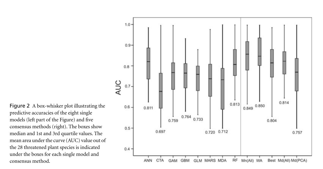
Anderson et al. assess the utility of consensus based predictors in species distribution models. These consensus predictors are made up of a number of fitted species distribution models of varying types. Component SDMs used for consensus modeling were GLM, GAM, MARS, ANN, GBM, RF, CTA, and MDA. These individual models were trained and evaluated on appropriate sub-subsets of the 70% training data subset in order to pre-evaluate these models for the purpose of consensus modeling. Consensus models assessed include Median(All) and Mean(All) which use the median and mean, respectively, of the predictions of all 8 models. The WA approach determines the 4 models with highest accuracy for a given species and computes a weighted average of their outputs. Median(PCA) is calculated as the median of the 4 models for which the variance of the predictions along the 1st principle component of a PCA was the greatest. Finally, Best simply selects the best individual model based on the highest pre-evaluated AUC value. Each of these methods, as well of each of the individual models, were then evaluated using the 30% testing data subset. WA and Mean(All) provided significantly more robust predictions than all single models and all other consensus methods. WA was the best model with a mean AUC of .850 and better predictive performance than all single-models on 21 of 28 species. These methods provide a functional alternative to thorough single-model evaluation and comparison. The fact that the true consensus models consistently outperform the “Best” consensus model suggests the utility of these methods over comparative evaluation. These consensus models also effectively address the common issues that some single-models provide better predictions for interpolation and some for extrapolation and that the best evaluated model often varies significantly from species to species.


Anderson figure

Invasive species distribution modeling (iSDM): Are absence data and dispersal constraints needed to predict actual distributions?

Václavík, T. and R. K. Meentemeyer (2009). “Invasive species distribution modeling (iSDM): Are absence data and dispersal constraints needed to predict actual distributions?” Ecological Modelling 220(23): 3248-3258.

http://www.sciencedirect.com/science/article/pii/S0304380009005742

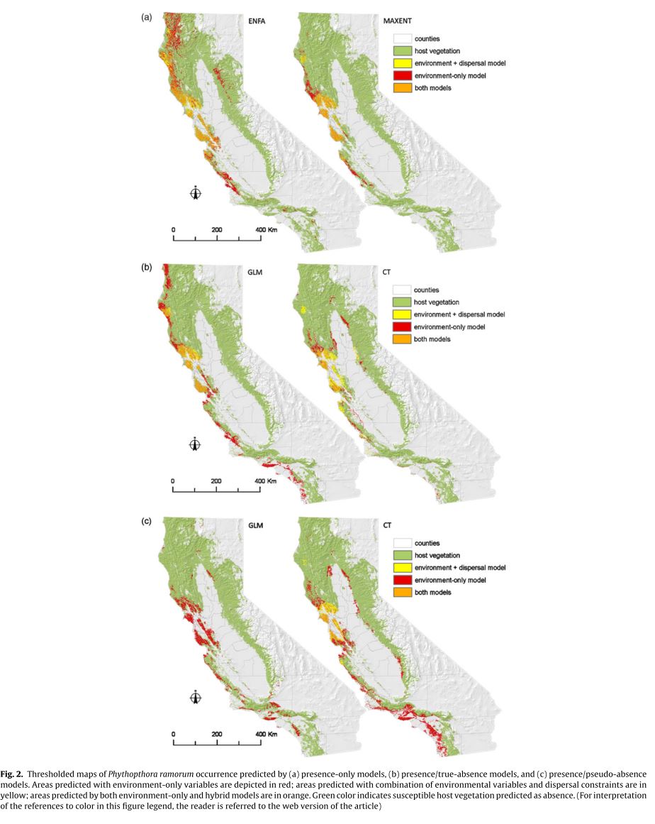
Vaclavik and Meentemeyeer focus on the specific problem of modeling the distribution of an invasive species in the process of invading across a landscape. iSDM forces the modeler to address the likely generally common problem of dispersal limitations because there will necessarily be a number of locations across the landscape which are environmentally suitable but currently inaccessible to the species. This paper examines how the addition of a measure of dispersal to iSDMs will affect the performance of models, alongside an attempt to determine the differences in performance of models trained using presence-absence, presence-psuedoabsence, and presence-only data respectively. The authors perform this analysis using Phytophthora ramorum an invasive generalist pathogen responsible for sudden oak death. 890 field plots were exhaustively sampled for evidence of the pathogen in the summers of 2003, 2004, and 2005, providing a reliable presence-absence data set. A number of pseudoabsences, points randomly chosen that could potentially be inhabited by the pathogen but which were not sampled, equal to the number of verified absences was also generated. Eight environmental variables were used to fit models including a spatial distribution of the key infectious host of the pathogen. All models were trained either exclusively on these environmental variables or on these variables and a measurement of “force of invasion” at a given point. Force of invasion was modeled using the following equation:

where djk is the Euclidean distance between each potential source of invasion k and the target plot i. The parameter a determines the shape of the dispersal kernel where low values of a indicate high dispersal limitation, and can only be estimated from presence-absence data. For models trained without true absence data a simpler force of infection metric based exclusively on the above-mentioned Euclidean distances is used. Two models using just presence-only data (ENFA, and MaxEnt) and two using presence-absence or presence-pseudoabsence (GLM and CT) were used. GLM and CT based on presence-absence data, including dispersal constraints were the highest performing models. The inclusion of dispersal constraints significantly increased the performance of most models. Without dispersal constraints presence-only models outperformed the other types of models (though this phenomenon was clearly driven by the good performance of MaxEnt). Presence-only models generally predicted larger areas of invasion than both presence-absence and presence-pseudoabsence but all models showed a clear reduction in predicted area when dispersal constraints were included. This paper clearly illustrates the importance of including probability of dispersal into SDMs for species in the process of invading a landscape. The estimates of “force of dispersal” seem as if they would suffer substantially from any sort of bias in the sampling of presence points but they may have been able to account for this in their sampling strategy. It would be interesting and useful to determine how these concepts could be applied to non-invasive species which nonetheless have dispersal restrictions preventing them from accessing some favorable areas of a landscape, allowing us to generally relax the assumption of equilibrium of distribution across the landscape. Such applications would likely require a more complex estimation of force of dispersal. In these closer to equilibrium cases there are likely landscape features which significantly slow the rate of dispersal across certain areas, which in turn creates the pattern, so we cannot assume an even rate of dispersal over time and space.


vlacivik figure

Classification in conservation biology: A comparison of five machine-learning methods

Kampichler, C., Wieland, R., Calmé, S., Weissenberger, H., & Arriaga-Weiss, S. (2010). Classification in conservation biology: A comparison of five machine-learning methods. Ecological Informatics, 5(6), 441–450. http://doi.org/10.1016/j.ecoinf.2010.06.003


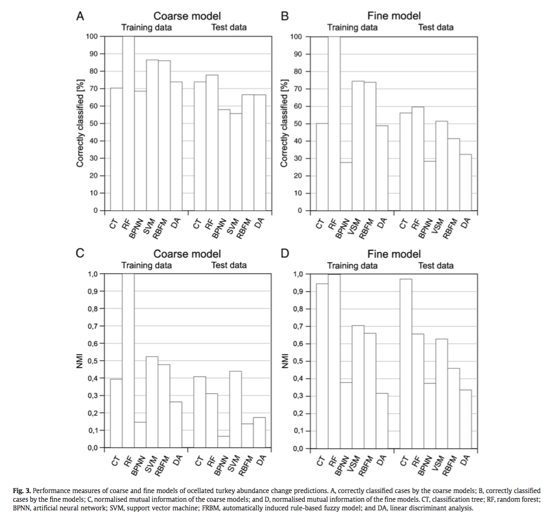
Machine learning methods have recently been adopted by ecologists to use in classification (eg. bioindicator identification, species distribution models, vegetation mapping) and there is an increasing amount of literature comparing the strengths and weaknesses of different machine learning techniques over a variety of applications. Kampichler et al add to this base of knowledge by comparing five machine learning techniques against the more conventional discriminant function analysis in their application to an analysis of abundance and distribution loss of the ocellated turkey (Meleagris ocellata) in the Yucatan Peninsula. They used data on turkey flock abundance (including absences) from the study area and 44 explanatory variables, including prior turkey abundance in local and regional cells, vegetation and land use types, and socio-demographic variables.

The techniques investigated were
– Classification trees (CT): uses a binary branching tree to describe the relationships between explanatory and predictor variables
– Random forests (RF): constructs many trees and then bags the trees to select the explanatory variables
– Back-propagation neural networks (BPNN): creates a network whose nodes are weighting by the training data
– Automatically induced fuzzy rule-based models (FRBM): processes variables based on algorithms using fuzzy logic
– Support vector machines (SVM): maps training data into an n-dimensional hyperplane and applies a kernel function to maximize seperation between the classes
– Discriminant analysis (DA): combines the explanatory variables linearly in an effort to “maximize the ratio between the separation of class means and within-class variance”

They compared the techniques based on their ability to correctly classify training and test data and using the normalized mutual information criterion, which is based on the confusion matrices and measures similarities between predictions and observations from 0 (random) to 1 (complete correspondence). In general, RF and CT performed the best, however the authors ranked CT first because of its high interpretability. An interesting point brought up is the fact that, in spite of the recent influx of machine learning in the scientific literature, most conservation decisions do not consider their results, most likely because of the lack of their interpretability and expertise needed to optimize the models. With this in mind, SVM, which performs relatively well, may not be the appropriate choice for conservation management because they are not well understood by ecologists lacking the proper mathematical training.

Screen Shot 2016-02-21 at 3.57.18 PM


Screen Shot 2016-02-21 at 3.57.45 PM

AUC: a misleading measure of the performance of predictive distribution models

Lobo, J. M., Jiménez-Valverde, A., & Real, R. (2008). AUC: a misleading measure of the performance of predictive distribution models. Global Ecology and Biogeography, 17(2), 145–151. http://doi.org/10.1111/j.1466-8238.2007.00358.x


With the increase in the use of predictive distribution models, especially with regards to species niche modeling, many are turning to the the area under the receiver operating characteristic curve (AUC) to assess the predictive accuracy of the models. Lobo et al have five main issues with the use of AUC in this manner. According to Lobo, AUC…

1) is insensitive to transformations of predicted probabilities, if ranks are preserved, meaning that models that are well fit may have poor discrimination and vice versa
2) summarizes test statistics in areas of extreme false-positive and –negative rates that researchers are rarely interested, leading the authors to suggest partial AUC
3) weights omission and commission the same. In the case of presence-absence data, false absences are more likely than false presence data, therefore their respective errors are not equal
4) plots do not describe the spatial distribution of errors, which would allow researchers to examine whether errors are spatially heterogeneous
5) does not accurately assess accuracy if the environmental range is larger than the geographical extent of presence data, as is the case for most SDM predictions

Additionally, AUC is often used to determine a ‘threshold’ probability of species distribution when converting a SDM to a binary, in spite of the fact that a ‘benefit’ of AUC is it is independent of the chosen threshold, and its corresponding subjectivity. The only instance in which the authors encourage use of AUC is in distinguishing between species whose distribution is more general (low AUC score) vs restricted. In order to combat the failings of AUC, Lobo et al suggest that sensitivity and specificity also be reported and that AUC only be used to compare models of the same species over an identical extent. I think another important point to include would be the quality of data. A cause of several of these problems is the bias of absence data in species distributions, and extra effort to combat this bias and ensure more complete presence-absence data sets would reduce the bias introduced by AUC.

Not as good as they seem: the importance of concepts in species distribution modeling

By comparing existent models, some ecologists found that complicated modeling techniques are more robust in terms of realized distribution modeling, and that predictions are usually more reliable for the species with smaller range sizes and higher habitat specifity. Jimenez-Valverde, Lobo, and Hortal argued that the interpretation of modeling results found in the comparisons above would vary if methodological and theoretical considerations are taken into consideration. They mentioned three important topics that need to be taken into consideration when conducting species distribution modeling: 1) the distribution between potential and realized distribution, 2) the effect of the relative occurrence area of the species on the results of the model performance, and 3) the inaccuracy of the resulted prediction of the realized distribution from different modeling methods. They reviewed most recent papers applying SDMs and discuess the negative implications of neglecting the three issues mentioned above, targeting on two general conclusions from other comparison papers:

– Are complex techniques better for the prediction of species distributions than simple ones?

With the bias shown by most of the biodiversity inventories, any comparisons among presence-only modeling generally provide distribution close to the potential. A more complex technique tends to overfit the presence data. When validate it with true absence data, it can be erroneously concluded that the predictions from the complex one are more accurate.

– Are the predictions fro specialist species more reliable than for generalists?

Jimenez-Valverde et.al. argued that the seemingly better predictions for specialists are usually the result of the properties of the data used for validation. Besides, rare/specialists and common/generalists gradients are extent- and scale- dependent. They found models of rare species are inevitably with high discrimination, which would be either over or underestimate the distribution of the species.

Their conclusion is that a solid conceptual and methodological framework is necessary for future works evaluating, comparing, and applying species distribution modeling techniques. This paper is inspiring since it provided alternative explanations for universally admitted conclusions. It will be more convincing that they can have species example as supports for their theoretical arguments. In addition, they “deliberately avoided using the term niche to refer to species distributions” due to the recognition that species can be absent from suitable habitat and/or present in unsuitable ones. So they clarified that they were only talking about statistical models, which are not able to provide a description if species niche. It is kind of ironic that they supported a “better understanding of basic concepts for any species modeling or methods comparison” on one hand, and avoided to talk about the most basic concepts behind distribution theory on the other hand.

Evolutionary diversification, coevolution between populations and their antagonists, and the filling of niche space

Ricklefs, R. E. (2010). Evolutionary diversification, coevolution between populations and their antagonists, and the filling of niche space. Proceedings of the National Academy of Sciences, 107(4), 1265–1272. http://doi.org/10.1073/pnas.0913626107

It is difficult to think about ecological niches without considering the consequences for species coexistence and biodiversity. Stemming from this is the idea of “niche filling”, in that a finite niche exists and because one species is already “filling” it, another cannot persist in the same niche at the same geographical location. This has led to the theory of an equilibrium number of niche spaces, whereby diversification in one clade is balanced by a decrease in diversity in other clades. Ricklefs tested this hypothesis by analyzing several datasets of bird clade diversity and range sizes, predicting that if the hypothesis holds true, the total niche space per clade would scale with the species diversity. His results found that this was not the case, predicting this independence of niche space may be due to higher clade overlap and smaller niche space for individual species within high-diversity clades. The constraint on niche space, Ricklefs proposes, may be caused by the coevolution of pathogens. As pathogens co-evolve with their host, they keep the niche space of one particular species from expanding too broadly, thereby allowing for a higher diversity of closely related species. In the field of niche theory, the inclusion of pathogens is novel, as the ‘boundaries’ of niche space are conventionally defined by competition interactions or resource limitation. The inclusion of both pathogens and co-evolutionary dynamics in the defining of a species niche space represents an important, although somewhat daunting, step towards a further understanding of niche theory. Ricklef’s theory is based on the idea that ‘diversity begets diversity’ evolutionarily and that pathogens are host-specific and respond to the co-evolutionary arms race, otherwise known as the Red Queen Hypothesis, by host switching, and I am doubtful how often this is seen in nature.