In defense of ‘niche modeling’; ‘Niche’ or ‘distribution’ modeling? A response to Warren

These papers discuss and argue the terminology used to describe the process of determine where species are able to inhabit.  Specifically the use of the terms Ecological Niche Models and Species Distribution Models to describe the techniques used to determine where or potentially where species are able to inhabit.

Warren (2012) criticizes the “loss” of the niche in the terminology.  While he sympathizes that many of these models are trained using data that only comes from the distribution of a species, he also argues that the underlying assumption of these models is that they are estimating the niche. The argument that these environmental predictors have some effect on biological processes of the organism and that often these models omit processes (e.g. dispersal).  Here, he defines the niche as the “conditions within which the species can survive and reproduce”. He suggests we continue to acknowledge the conceptual framework being used and the we are attempting to estimate the niche in our research.

In a response to Warren, McInerny and Ettienne (2013) defend the position of using ‘distribution’ to describe the techniques.  They criticize his definition (even the definitions he provides, pointing out that he invokes two ones)  of niche saying it constrains the selection of predictor variables to ones that are only biological.  However, they point out that these problems have also been considered with the SDMs through parameter selection, model structure, and functional forms.  Lastly, the point out that other words could also be used to describe these models (“habitat suitability”, “bioclimate envelopes”, “resource selection”) but they stand by the choice of the neutral words “species distribution modeling”.

Warren, D. L. 2012 In defense of ‘niche modeling’. Trends Ecol. Evol. 27, 497–500. doi:10.1016/j.tree.2012.03.010

McInerny, G. J. & Etienne, R. S. 2013 ‘Niche’ or ‘distribution’modelling? A response to Warren. Trends Ecol. Evol. 28, 191–192. http://dx.doi.org/10.1016/j.tree.2013.01.007

Scale-dependent role of demography and dispersal on the distribution of populations in heterogeneous landscapes


Motivation: Both dispersal and local demographic processes shape the distribution of the population among varying habitat qualities. However most theories, experiments, and field studies have focused on dispersal.  The authors attempt to show how both dispersal and demographic processes shape a population’s distribution, and when either mechanism is more important.

Population dynamics were primarily explained via demographic processes, while distribution was a function of dispersal process. These authors would also like to bring in the ideal free distribution (IDF) theory to explain population distributions.  IDF  predicts that individuals will be distributed among patches of different quality so that the fitness of individuals in different patches is equalized – individuals can’t improve fitness by moving to another patch. As an aside, given that the underlying theory requires individual choice of patch occupancy this work is only appropriate for populations that can actively choose how they are dispersed or move.  The IDF can arise from 2 possible mechanisms: 1) dispersal, where individuals use information about habitat quality to make movement decisions, or 2)  demographic processes where the habitat quality experienced by individuals affects demographic rates.

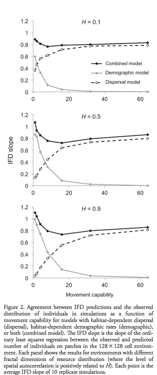
Methods:  The authors explore the 2 mechanisms that lead to IDF by extending a individual-based model of habitat dependent dispersal, growth, reproduction, and survival of individuals. All simulations wer done on a 128 x 128 cell grid. Each  grid/habitat patch had its own logistically growing resource, and patch quality differed by the carrying capacity of this resource. To examine the relative effects of dispersal and demography, the model simulations were run with only habitat dependent dispersal, habitat dependent demography, or both.   This was done by varying 2 traits: the maximum dispersal distance (M) and the spatial scale of resource heterogeneity (H).

Wk4Fig 2


Results: When both habitat dependent dispersal and demography were included in the simulation population distributions closely matched IFD predictions.   Simulations of populations with only demographic processes (i.e. Dispersal only) were overabundant in low-quality patches and under abundant in high-quality patches resulting in low correlation with IFD predictions. This effect was exacerbated in environments where the spatial scale of resource heterogeneity was large. When habitat quality influenced demographic rates (but dispersal was random), the effect of scale on IFD  was reversed – highly mobile populations were sub optimally distributed with respect to habitat quality, reducing the scale of resource heterogeneity only exacerbated the trend.

Take-home: Pulliam demonstrated the need to include passive dispersal processes when describing population distributions, Martin et al.  has demonstrated the need to include dispersal and demographic processes of populations with active dispersal. Spatial scales that limited the resource matching capacity of one process coincide with those that promoted the resource matching capacity of the other process.


Martin, Benjamin T., et al. “Scale‐dependent role of demography and dispersal on the distribution of populations in heterogeneous landscapes.”Oikos (2015).  doi: 10.1111/oik.02345

Not as good as they seem: the importance of concepts in species distribution modeling

By comparing existent models, some ecologists found that complicated modeling techniques are more robust in terms of realized distribution modeling, and that predictions are usually more reliable for the species with smaller range sizes and higher habitat specifity. Jimenez-Valverde, Lobo, and Hortal argued that the interpretation of modeling results found in the comparisons above would vary if methodological and theoretical considerations are taken into consideration. They mentioned three important topics that need to be taken into consideration when conducting species distribution modeling: 1) the distribution between potential and realized distribution, 2) the effect of the relative occurrence area of the species on the results of the model performance, and 3) the inaccuracy of the resulted prediction of the realized distribution from different modeling methods. They reviewed most recent papers applying SDMs and discuess the negative implications of neglecting the three issues mentioned above, targeting on two general conclusions from other comparison papers:

– Are complex techniques better for the prediction of species distributions than simple ones?

With the bias shown by most of the biodiversity inventories, any comparisons among presence-only modeling generally provide distribution close to the potential. A more complex technique tends to overfit the presence data. When validate it with true absence data, it can be erroneously concluded that the predictions from the complex one are more accurate.

– Are the predictions fro specialist species more reliable than for generalists?

Jimenez-Valverde et.al. argued that the seemingly better predictions for specialists are usually the result of the properties of the data used for validation. Besides, rare/specialists and common/generalists gradients are extent- and scale- dependent. They found models of rare species are inevitably with high discrimination, which would be either over or underestimate the distribution of the species.

Their conclusion is that a solid conceptual and methodological framework is necessary for future works evaluating, comparing, and applying species distribution modeling techniques. This paper is inspiring since it provided alternative explanations for universally admitted conclusions. It will be more convincing that they can have species example as supports for their theoretical arguments. In addition, they “deliberately avoided using the term niche to refer to species distributions” due to the recognition that species can be absent from suitable habitat and/or present in unsuitable ones. So they clarified that they were only talking about statistical models, which are not able to provide a description if species niche. It is kind of ironic that they supported a “better understanding of basic concepts for any species modeling or methods comparison” on one hand, and avoided to talk about the most basic concepts behind distribution theory on the other hand.

The vulnerability of species to range expansions by predators can be predicted using historical species associations and body size

The vulnerability of species to range expansion by predators can be predicted using historical species associations and body size. Declines in abundance in local extinctions are the direct consequence of climate exceeding physiological tolerances in addition to the indirect consequences of climate change on species interaction. These indirect impacts of climate change and biodiversity are more difficult to predict or observed when compared to the physiological impacts.

Species ranges have changed at variable rates under climate change, potentially making novel ecosystems. However, species expanding their range can encounter resident prey, predators and competitors that were present in their historical range (i.e. species historically occurred in some patches). The ecological niche concept has been used to understand patterns of co-occurrence and species interaction; this could also be a useful tool to protect the indirect impacts of climate change.

Here, the authors suggest using species associations and body size as a simple measure of the impacts of species introductions facilitated by climate change. Negative associations can indicate strong ecological interactions including competitive exclusion, predation or it could indicate different abiotic requirements. Functional traits often mediate the strength of species interactions – which can be used to infer niche differences. Body size is correlated with many functional traits (i.e. reproductive rate, dispersal ability, diet breadth and or predation). Increased differences in body sizes would indicate decreased competition, while the ratio of predator to prey body size indicates strength of predation.

The authors hypothesize that pairwise species associations and body size can predict the relative risk imposed on resident species by predators whose ranges are expanding. They focus centrarchid predators undergoing range expansion in the Great Lakes region. This expansion is expected to be problematic since these predators are not often found in smaller lakes with the potential prey species. The question then becomes whether this negative species associations are good predictors of vulnerability, and how resident species body size impacts the risk associated with additional predators.

Methods: The data set consisted of 1551 links with paired historical and contemporary species samplings. A total of 106 fish species were observed which was then used to create presence absence data pairs in 2 x 2 contingency tables. The Phi– coefficient was calculated for these 2 x 2 tables (range from -1, 1) the relative risk ratio was then calculated on the tally of lakes where the resident species was absence after the introduction of the predator.

Results:  Centrarchid introductions significantly increase the likelihood of some prey species loss, while protecting loss of native centrarchids based on introduction data. Historical species associations were a strong predictor of the introduced species’ impact. Additionally, resident species total length was a significant indicator of the relative risk ratio.

Take home:  Traits mediate species interactions, and body size is an easily measurable trait that is correlated to many other traits in fish species. Body length and historical species associations can be used to forecast the impact of introduced species on the native species under climate change.

Given that fish can have convoluted food webs, using body size as a proxy of competition and predation seems like a very elegant solution.


Alofs, Karen M., and Donald A. Jackson. “The vulnerability of species to range expansions by predators can be predicted using historical species associations and body size.” Proc. R. Soc. B. Vol. 282. No. 1812. The Royal Society, 2015. http://dx.doi.org/10.1098/rspb.2015.1211


Climatic Niche Shifts Are Rare Among Terrestrial Plant Invaders

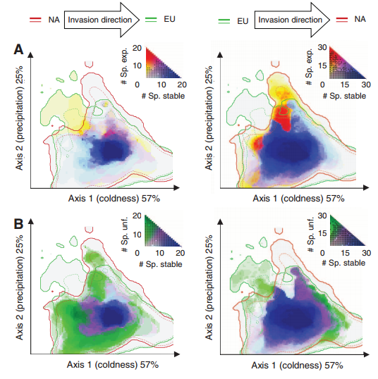
Species may be able to shift their climatic niche requirements according to some researchers, while most models of diversity as a function of global change assume a constant climatic niche for a given species. This is especially the case in species invasions, where the species may be able to exist in climates different from the native range. The authors examined 50 invader plant species in North America and Eurasia in order to quantify the degree of niche expansion, niche overlap, and niche unfilling (species only partially fills its native niche in the invaded range). They found niche conservatism in 46% of the plant species, suggesting that plants largely occupy similar niches in their invaded range. Further, the authors found that when niche expansions were present, 14% of these species show greater than a 10% niche expansion, which they argue is rather low. Niche unfilling was rather common (48% of species), though they don’t discuss the influence of dispersal limitation or the influence of time since invasion on this result. One would think that recent invaders that haven’t had time to disperse (or those under active control) would not have time to reach the extent of their niche, which would appear as niche unfilling compared to their niche in the native range. In their supplement, the authors detail how they calculated the E-space used to quantify niche overlap (a standard PCA whose first two axes explained 82% of the variation in 8 variables including degree day, evapotranspiration coefficients, temperature and precipitation).

Link to paper

Supplement here 

Facilitation and the niche: implications for coexistence, range shifts and ecosystem functioning

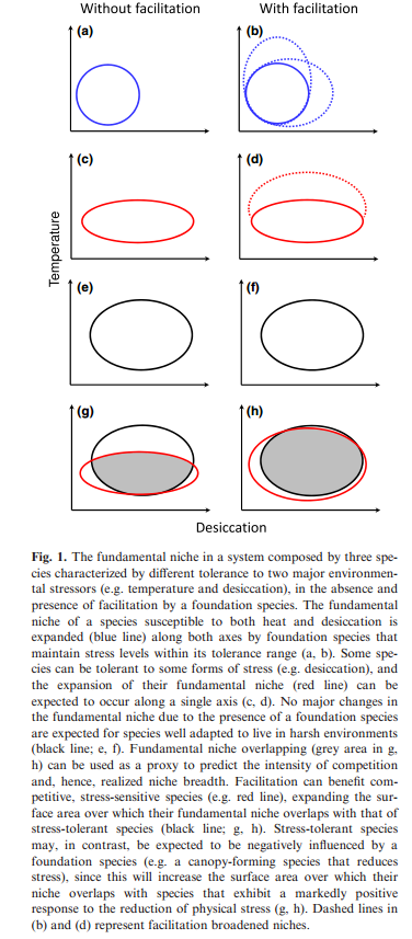
The original description of the niche purposefully excluded the impact of species interactions for niche determination. In a more applied context, several authors have included species interactions, specifically negative interactions, in determining a species niche or geographic range. Here, the authors consider the effect of facilitatory interactions on the expansion of the niche. An example would be if the presence of another species created habitat necessary for the colonization of a secondary species, such as the case with woodpeckers facilitating the presence of tree hole dwelling insects. Species interactions could create suitable environments (e.g., microhabitat variation; see Chesson (2000)) or provide access to a resource that could enable persistence. The authors argue that the introduction of a facilitatory species could result in a niche shift of a focal species in E-space (as in Figure 1). The authors also discuss the role of coexistence when competing species are both responding to a facilitatory species. They argue that niche broadening as a function of facilitation may promote exclusion of one of the species, as niche broadening may put two species in competition where they previously weren’t. This will only be a big issue when fitness differences are large.

Link to paper

Chesson, P. (2000a) Mechanisms of maintenance of species diversity. Annual Review of Ecology and Systematics, 31, 343–366

Environmental data sets matter in ecological niche modelling: an example with Solenopsis invicta and Solenopsis richteri

Authors: Peterson and Nakazawa

DOI: http://10.1111/j.1466-8238.2007.00347.x

This study highlights the potential effects environmental data can have on model results. The study system selected by researchers was assumed to be a matured species invasion of fire ants where experts were confident that the invading species was approaching its range limit. Researchers compared six different environmental data sets with a genetic algorithm rule-set prediction (GARP) for model development. The different types of rainfall data sets considered were the following: WC1, WC2, IPCC, CCR, and NDVI. GARP operates by sampling available occurrence points (with replacement) to build a population of a set number of presence points, and then an equal number of sampled points of no occurrence. Both sets of occurrence/no-occurrence are then divided equally into training and testing data sets. A drawback to this study is that comparisons are made only qualitatively by depicting predictive differences through mapping, and no quantitative measure of model performance is provided. It is clear from the results offered that different environmental data sets can yield differences in model prediction, yet the authors provided little speculation on possible reasons for such differences.

Vacated niches, competitive release and the community ecology of pathogen eradication

Lloyd-Smith JO. 2013 Vacated niches, competitive release and the community ecology of pathogen eradication. Phil Trans R Soc B 368: 0120150. http://dx.doi.org/10.1098/rstb.2012.0150

This article reviews whether it is sensible to consider the niche left behind when a pathogen is eradicated, and to worry about the risk that this niche will be recolonized by another pathogen causing a similar disease. This topic is highly controversial in the epidemiological literature regarding he merits of eradication. Lloyd-Smith proposes the term ‘vacated niche’ to describe the pathogen niche left behind following a successful eradication effort and evaluates evidence claiming that vacated niches can alter the epidemiology of the surrounding community of pathogens. Potential mechanisms of competitive release or evolutionary adaptation can elevate the health burden from other pathogens (i.e. resulting in increased incidence of another pathogen). However, he emphasizes that a vacated niche will not necessarily cause emergence of a replacement pathogen, or that any such pathogen will have similar disease characteristics to the eliminated one. He concludes that the vacated niche is an opportunity for other pathogens, but many factors will determine whether and how they may capitalize on it. This article is an expansion to the ecological discussion of whether empty niches actually exist and it is interesting to think about how these concepts would lend themselves to invasive species and/or local species extinctions.

Demographic compensation among populations: what is it, how does it arise and what are its implications?

Villellas, J., Doak, D. F., García, M. B., & Morris, W. F. (2015). Demographic compensation among populations: what is it, how does it arise and what are its implications? Ecology Letters, 18(11), 1139–1152. http://doi.org/10.1111/ele.12505

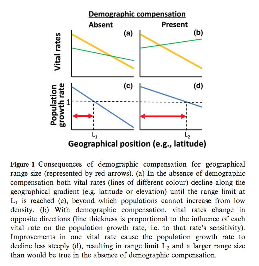
A common assumption in the analysis of species distributions across an environmental gradient are that vital rates decline across the gradient as they approach the range limit. Villellas et al. aimed to investigate an opposing theory, demographic compensation (DC), in which mean population vital rates change in opposing ways across spatial or environmental gradients. Using a randomization procedure, they tested for the presence of DC across 26 plant demographic studies, based on the assumption that DC would lead to more negative correlations among vital rates than expected by chance. They found both that there were more positive and more negative correlations than expected by chance, suggesting that the overall tendency is for vital rates to respond similarly, but that DC is a phenomenon that does exist. Investigating further, this pattern was driven by fecundity and recruitment rates, which had the highest proportion of negative correlation amongst vital rates and to which the population growth rate had high variance and sensitivity, respectively, evidence that DC acts by influencing vital rates as different life stages. For those studies that showed evidence of DC, another randomization procedure was done to compare the variation of population growth rates with a nd without DC, finding that DC halved the variance in population growth rates. This has important implications for SDM, as high growth rate variation at the range limits of species distributions can lead to a higher rate of stochastic extinctions, perhaps influence presence data and the probability of persistence in these limits. If we are to believe that DC is at play, however, there will be less variation at the range limits, implying that the ‘e-space’ may be closer to Hutchinson’s binary persistence-extinction demarcations than originally thought.

Screen Shot 2016-02-01 at 6.05.08 PM

Five (or so) Challenges for Species Distribution Modeling

The authors present 5 challenges for SDM.   By confronting these models, we should be able to generate better and provide a better understanding of  these models.

  1. Clarification of the niche concept: The authors suggest a diversion from the Hutchinson definition of the niche (n-dimensional hyper-volume of environmental variables) to more of a Grinnellian definition: the set of environmental conditions at which the birth rate of the population is greater than or equal to the death rate.  They also point out the need for the clear(er) distinction between potential habitats for species (ranges/areas that the conditions are “right” for a species to inhabit) and potential geographic distributions of species (incorporates spatial factors such as dispersal)
  2. Improved designs for sampling data for building models: Models are sensitive to bias. Subsampling datasets are likely to remove or reduce biases. A (more expensive) alternative is to target specific, strategic additional sampling locations.
  3. Improved parameterization strategies: Different parameterizations of models can result in vastly different projections of species distributions.  We to better understand why and when different parameterizations of the same technique provide different results.
  4. Improved model selection and predictor contribution: There are many different strategies that can be used to compare different models. However, finding the individual contribution of each predictor is a more difficult problem.  Further testing of proposed solutions provided by the authors is needed.
  5. Improved model evaluation strategies: Evaluation of models can be discussed in the light of three different implementations: explanation, understanding and prediction. Typically modelers use the “wrong” evaluation tool outside of the scope of their goal or question. They present two different forms of evolution: verification (projecting using an new/independent set of data) and validation (maximizing the fit to training data).

Araújo, M. B. & Guisan, A. 2006 Five (or so) challenges for species distribution modelling. J. Biogeogr. 33, 1677–1688. (doi:10.1111/j.1365-2699.2006.01584.x)